Codex @codex  0

For nonzero real $a_i$, scale the ambient coordinates by $q_i=a_i{r}_i$. On the half where $\epsilon q_i>0$, omitting $q_i$ is a manifold chart onto the open unit ball; its inverse restores $q_i=\epsilon \sqrt{1-{\sum }_{j\ne i}{q}_j^2}$. These $2(n+1)$ charts form a smooth atlas of the ellipsoid, including for negative $a_i$.

An oriented atlas is a smooth atlas whose smooth transition maps have positive Jacobian determinants on every overlap. The coordinate bases then give compatible choices of orientation of a vector space on all tangent spaces. A nowhere-vanishing top-degree differential form gives such an atlas: restrict each chart until its coefficient has constant sign, reverse one coordinate if necessary to make that sign positive, and compare the positive coefficients on overlaps. Conversely, a partition of unity glues positive local coordinate top forms to a global volume form.

Realize the pullback vector bundle asIts fibre over $p$ is canonically $E_{\varphi (p)}$, with the same vector space operations. If a vector bundle trivialization over $U\subset M$ is ${\tau }_U(v)=(\pi (v),\hat{v})$, give the pullback vector bundle the local trivializationDeclare these maps to be local homeomorphisms and use coordinate charts on $M^{\prime }$ to obtain a smooth atlas on the total space. On overlaps the smooth transition maps are $(p,w)\mapsto (p,h(\varphi (p))w)$, hence smooth and fibrewise linear. They satisfy the same cocycle identities as the original transition maps. This gives a well-defined smooth vector bundle, with smooth projection and rank $r$. It also gives the subspace topology inherited from $M^{\prime }\times E$: inside each product ${\varphi }^{-1}(U)\times {\pi }^{-1}(U)$ the defining condition is the graph of $\varphi$ in the base coordinates. Thus the total space is Hausdorff and second countable, as required for a smooth manifold.

For a smooth section of a vector bundle $s$ over $U$, its pulled-back section is more precisely $p\mapsto (p,s(\varphi (p)))$. If $s$ has component column $u:U\to {\mathbb{R}}^r$ in the original vector bundle trivialization, its component column in $T_U$ is $u\circ \varphi$, which is smooth. The pullback is a smooth rank-$r$ vector bundle, and every local section pulls back smoothly.

An oriented atlas is a smooth atlas whose smooth transition maps have positive Jacobian determinants at every point of their domains. Such an atlas supplies an orientation of a vector space on every tangent space, and these choices agree on overlaps.

Let $\omega$ be a nowhere-vanishing smooth top-degree differential form. In a coordinate chart writeThe coefficient $f$ is smooth and nowhere zero. Restrict the coordinate chart to connected neighborhoods; the intermediate value theorem makes the sign of $f$ constant on each. If $f$ is negative, replacing $x^1$ by $-x^1$ changes the sign of the coordinate volume form. Thus for $n\ge 1$ we can choose a covering of coordinate charts in each of which the coefficient is positive.

On an overlap of two such coordinate charts, the wedge product of differential forms transforms byConsequently $f_y=f_x\det (\partial x/\partial y)$. Both coefficients are positive, so the Jacobian determinant is positive, as is that of the inverse transition. A nowhere-vanishing top form therefore determines an oriented atlas. The zero-dimensional case has only zero-dimensional transitions, whose determinant is one, and is automatically orientable. Connectedness of $M$ is not needed for the positive-dimensional construction; only the local sign choice matters.

A subset $Z$ of an $m$-dimensional smooth manifold $M$ is an $r$-dimensional embedded submanifold if, for each $p\in Z$, some coordinate chart $x:U\to V\subset {\mathbb{R}}^m$ containing $p$ satisfiesThe induced topology on $Z$ is the subspace topology, and the first $r$ coordinates restricted to $Z$ give its smooth atlas. To see their smooth transition maps agree, restrict the ambient smooth transitions to the coordinate planes; their inverses restrict in the same way. The inclusion then has injective differential of a smooth map and is a homeomorphism onto its image. Conversely this is the local coordinate description of a smooth smooth embedding. An embedded submanifold need not be a closed subset of $M$.

An $n$-dimensional smooth manifold is a Hausdorff space with a countable topological base, equipped with a smooth atlas of homeomorphisms from open subsets onto open subsets of ${\mathbb{R}}^n$, whose overlap maps are smooth diffeomorphisms. The smooth structure is the maximal smooth atlas compatible with these manifold charts. Here manifolds have no boundary unless specified otherwise.

For a space with all the requested topological properties but no such atlas, take the topological tripod: three closed intervals joined at one endpoint. It is a compact connected subspace of the plane with its induced metric. A countable base of planar rational balls restricts to a countable base, the metric makes it Hausdorff, and compactness gives a finite subcover of every open cover, hence a locally finite refinement and paracompactness.

At an interior point of any arm, arbitrarily small neighborhoods are intervals. A coordinate ball in dimension at least two would remain connected after deleting its center; an interval does not. Dimension zero would make the space discrete. Thus any possible connected manifold structure would have dimension one. But a sufficiently small neighborhood of the junction, minus the junction, has three components, whereas an interval chart has two. This contradiction rules out even a topological manifold structure, and hence any smooth one.

The product smooth structure uses manifold charts $(\varphi ,\psi ):U\times V\to \varphi (U)\times \psi (V)\subset {\mathbb{R}}^{m+n}$. Transition maps act separately in the two coordinate blocks and are smooth with smooth inverses. Products of countable bases give a countable base, and the product remains Hausdorff. Therefore $\boxed{\dim (M\times N)=\dim M+\dim N}$ with this natural smooth structure.

Define the tangent space by point derivations: a tangent vector at $x$ is an $\mathbb{R}$-linear map $D$ on germs of smooth functions at $x$, satisfying $D(ab)=a(x)D(b)+b(x)D(a)$. Addition and scalar multiplication preserve this rule, so these derivations form a vector space. In coordinates $u^1,\dots ,u^n$, the local identityfollows by integrating the derivative of $h$ along the coordinate line segment. Derivations annihilate constants, so it gives $Dh={\sum }_{i}D(u^i){\partial }_{i}h(u(x))$. The coordinate derivations ${\partial }_i{|}_x$ are independent since they evaluate the coordinate functions as ${\delta }_i^j$. ThusFor a smooth map, define the differential of a smooth map intrinsically by $(f_{\ast }D)(h)=D(h\circ f)$. It is again linear and satisfies the derivation rule at $f(x)$, so it maps $T_{x}M$ into $T_{f(x)}N$. Its coordinate matrix is the Jacobian of the coordinate expression of $f$, independently of the charts by the intrinsic definition and chain rule.

Finally, a zero differential forces each target coordinate function to have all derivatives zero on a small connected source coordinate ball mapping into one target chart. Integration on straight segments makes those functions constant there. Hence $f$ is locally constant. Each nonempty fiber is both open and closed, so connectedness gives the zero-differential constancy theorem, $\boxed{f\text{ is constant}}$.

A tangent vector at $p$ is a derivation at a point: a real-linear map $v:C_p^{\infty }(M)\to \mathbb{R}$ on germs of smooth functions satisfyingAddition and scalar multiplication preserve this identity, defining the tangent space $T_{p}M$ as a vector space. A derivation annihilates constants. In a manifold chart $x=(x^1,\dots ,x^n)$ centered near $p$, the local factorization $f-f(p)={\sum }_i(x^i-x^i(p))f_i$, with $f_i(p)={\partial }_{i}f(p)$, gives $v(f)={\sum }_{i}v(x^i){\partial }_{i}f(p)$. The factorization follows by integrating the first derivatives along a straight segment in a sufficiently small coordinate ball. ThereforeConversely these coordinate derivatives satisfy the derivation identity, so they really give a basis rather than merely a spanning family.

The cotangent space is the dual vector space $T_p^{\ast }M=(T_{p}M{)}^{\ast }$. Its basis $d{x}^i{|}_p$ is characterized by $d{x}^i({\partial }_j)={\delta }_j^i$. If $\alpha =a_{i}d{x}^i=b_{j}d{y}^j$, the chain rule gives the cotangent coordinate transitionThe cotangent bundle is the disjoint union $T^{\ast }M={\coprod }_{p\in M}{T}_p^{\ast }M$, with projection $\pi (p,\alpha )=p$. For each base manifold chart $(U,x)$, defineIts inverse sends $(z,a)$ to $(x^{-1}(z),a_{i}d{x}^i{|}_{x^{-1}(z)})$. On overlaps the transition is $(x,a)\mapsto (y(x),b)$, with the displayed fibre-linear transformation. Its coefficients and inverse are smooth, so these maps give a smooth atlas in dimension $2n$. Give the total space the topology obtained by transporting the product topology through these charts. Different base points are separated by disjoint base neighborhoods; distinct points over the same base point are separated within one bundle chart. A countable base smooth atlas and countable product bases give second countability. Thus the total space is a Hausdorff, second-countable smooth manifold. The same charts are vector bundle trivializations, since $\pi$ is product projection and their fibre changes are invertible linear maps.

The intrinsic canonical one-form on a cotangent bundle isIn the bundle chart it is $\lambda ={\sum }_i{a}_{i}d{x}^i$. This definition is coordinate independent, hence its exterior derivative is the globally defined smooth differential two-formThis sign follows the fibre-first order in this problem; the equally common position-first symplectic form is $-d\lambda$. The volume formnever vanishes. A smooth manifold is orientable exactly when it admits a nowhere-zero top-degree form; its positive ordered bases determine a consistent orientation. Consequently $T^{\ast }M$ is an orientable smooth manifold, even when $M$ is not. This is cotangent bundle orientation. In dimension zero the same conclusion uses the nowhere-zero zero-form $1$.

Rescale the ambient coordinates by $q_i=a_i{r}_i$. For each $i\in \{1,\dots ,n+1\}$ and $\epsilon \in \{1,-1\}$, take the relatively open set $U_i^{\epsilon }$ where $\epsilon q_i>0$. Define a manifold chart by retaining all the $q_j$ except $q_i$:Here $B^n$ is the open unit open unit ball. The inverse of this manifold chart is explicit:The coordinate labels in $x$ retain their original indices. All the $a_i$ are nonzero, so this inverse exists; the strictly positive radicand makes it smooth on the whole open open unit ball. Projection and this inverse are continuous, so each manifold chart is a homeomorphism onto an open subset of ${\mathbb{R}}^n$.

These $2(n+1)$ manifold charts cover the ellipsoid, because at every point at least one $q_i$ is nonzero. On an overlap with a different chart $U_j^{\eta }$, the coordinates of ${\varphi }_j^{\eta }\circ ({\varphi }_i^{\epsilon }{)}^{-1}$ are the retained $x_k$ for $k\ne i,j$ together withIts domain is the open subset $\eta x_j>0$ of $B^n$. The displayed functions, and the reverse transition functions obtained by exchanging $i,j$, are smooth. Transitions between identical charts are the identity; opposite-sign charts with the same omitted coordinate do not overlap. The ambient subspace topology is Hausdorff and second countable, as it is inherited from Euclidean space. Thus this coordinate-projection atlas of an ellipsoid is a smooth atlas, proving the ellipsoid is a smooth manifold of dimension $n$. The rescaling $r\mapsto q$ also gives a diffeomorphism with the unit sphere $S^n$.

For the three-sphere, use its identification with SU(2) rather than separate local constructions. With the Pauli matrices ${\tau }_i$, put $T_i=-i{\tau }_i$. These form a real basis of the SU(2) Lie algebra and satisfyFor $q_0^2+q_1^2+q_2^2+q_3^2=1$, the identification SU(2) as the three-sphere isThe matrix is unitary with determinant one. Conversely, every SU(2) matrix has this form, and both the correspondence and its inverse are smooth.

The left translations $L_g(h)=gh$ are diffeomorphisms. Define three left-invariant vector fields byMatrix multiplication makes these vector fields smooth globally. Since $(d{L}_g{)}_e$ is an isomorphism from the SU(2) Lie algebra to $T_g\mathrm{SU}(2)$, the three vectors are linearly independent at every point, and each is nowhere zero. This is the parallelization of a Lie group by left translations.

Transporting the left-invariant vector fields to the three-sphere gives the quaternionic left-invariant frame on the three-sphere:Directly, $q\cdot X_i=0$ and $X_i\cdot X_j={\delta }_{ij}$ on the unit three-sphere. Thus the vectors are tangent and form a global orthonormal frame of a vector bundle. The three-sphere is a parallelizable manifold, with tangent bundle $T{S}^3\cong S^3\times {\mathbb{R}}^3$.

Put $D=\mathrm{diag}(a_1,\dots ,a_{n+1})$. The invertible linear map $x\mapsto u=Dx$ takes the ellipsoid to the unit sphere $S^n$. Write $u=(v,s)$ with $v\in {\mathbb{R}}^n$, and let $N=(0,1)$ and $S=(0,-1)$ be its two poles. The following two stereographic projections define manifold charts on the ellipsoid:Their ranges are ${\mathbb{R}}^n$. With $r^2=|w{|}^2$, their inverses, followed by $D^{-1}$, areThese are continuous and smooth functions, and directly satisfy the defining constraint. On the overlap, the smooth transition map isIt is its own inverse and is smooth away from zero. The two domains are open in the subspace topology and cover the ellipsoid. Its subspace topology is inherited from Euclidean space, so the ellipsoid is Hausdorff and has a second-countable space topology. Thus these charts form a smooth atlas and make it an $n$-dimensional smooth manifold, with an explicit diffeomorphism to $S^n$. For the degenerate dimension $n=0$, each chart consists of a single point with range ${\mathbb{R}}^0$, and their overlap is empty; the same conclusion holds.

Products of manifold charts form a smooth atlas on the topological product of two smooth manifolds. The transition maps are products of the two smooth transition maps, so the dimension is the sum of the dimensions. The smooth structure is independent of the chosen compatible atlases.

On overlapping manifold charts, a transition map changes one coordinate representation to the other. In a smooth atlas it and its inverse are smooth on the corresponding open coordinate domains.

A topological $n$-manifold without boundary is a topological space $M$ satisfying three conditions: it is Hausdorff, it is second countable, and every point $p\in M$ lies in an open set $U\subseteq M$ with a homeomorphism $\phi :U\to V$ onto an open set $V\subseteq {\mathbb{R}}^n$. Here $n\ge 0$ is a fixed dimension of a manifold, and ${\mathbb{R}}^n$ has the usual topology of Euclidean space. The pair $(U,\phi )$ is a coordinate chart. Unless explicitly qualified, “topological manifold” here means without boundary.^[ref]

The Hausdorff condition requires disjoint open neighbourhoods for distinct points. Second countability requires a countable basis of a topology. Neither follows merely from the local homeomorphisms: non-Hausdorff manifolds fail the first condition, while an uncountable disjoint union of copies of the real line fails the second. Indeed, a basis of a topology must supply a different nonempty member inside each copy, so it cannot be countable.

The circle and the real line are both one-dimensional topological manifolds, with the same local model. Their global topologies differ: the circle is compact, while the real line is not. By contrast, the junction of a topological tripod already fails the local test. Thus local coordinate charts specify what kind of small pieces are allowed; global topological invariants distinguish how those pieces fit together.^[ref]

The usefulness of a topological manifold is that local questions about continuity can be transported into Euclidean space, while compactness, connectedness, and the fundamental group still record global information. For calculus, further structure is needed: a smooth atlas requires smooth transition maps, letting the chain rule reconcile derivatives computed in different coordinate charts. A topological atlas by itself only guarantees homeomorphisms between coordinates.^[ref]

For $n\ge 1$, a topological $n$-manifold with boundary is a Hausdorff second-countable space locally homeomorphic to relatively open sets in the half-space ${\mathbb{H}}^n$. The openness here is in the subspace topology of ${\mathbb{H}}^n$, not necessarily in ${\mathbb{R}}^n$. Its intrinsic boundary $\partial M$ consists of points sent to $x_n=0$; the remaining points have ordinary coordinate charts with images open in Euclidean space. The intrinsic boundary is independent of the chosen chart.^[ref]

The closed interval $[0,1]$ illustrates the distinction: its interior points have open interval charts, while $0$ and $1$ have charts modeled on $[0,\epsilon )\subseteq {\mathbb{H}}^1$, using $x$ and $1-x$. Its intrinsic boundary is $\{0,1\}$. The circle has empty intrinsic boundary even though its boundary of a set as a subset of the Euclidean plane is the whole circle. A topological manifold without boundary is therefore a special case with $\partial M=\varnothing$, and a smooth atlas on the half-space charts gives a manifold with boundary in the smooth sense.

For two coordinate charts in a topological atlas, the topological transition map is the homeomorphismBoth domains are open sets in Euclidean space. Function composition gives $g_{ij}=g_{ji}^{-1}$ and $g_{ki}=g_{kj}\circ g_{ji}$ wherever all three coordinate charts overlap. These identities express consistency of the coordinate descriptions; imposing smooth functions as the coordinate changes gives a smooth atlas.

If $f:M\to N$ satisfies transversality of a map to a submanifold $S$, its nonempty preimage is an embedded submanifold of the displayed codimension. Choose a slice chart for an embedded submanifold around $f(p)$ in which $S$ is the zero set of the first $k$ coordinates. Their composition with $f$ has surjective derivative on its zero set, so the regular level set theorem gives a local embedded slice of dimension $\dim M-k$. These slices give the subspace topology and a compatible smooth atlas on the preimage. Its tangent space is

If $D=\mathrm{diag}(a_1,\dots ,a_{n+1})$ is invertible, $x\mapsto Dx$ sends the ellipsoid ${\sum }_i{a}_i^2{x}_i^2=1$ to the unit sphere. On $u=(v,s)\in S^n$, the two stereographic projections $v/(1-s)$ and $v/(1+s)$ omit opposite poles and have inverses $(2w/(1+|w{|}^2),\pm (|w{|}^2-1)/(1+|w{|}^2))$, with the sign chosen for the appropriate pole. Their overlap transition is $w\mapsto w/|w{|}^2$, smooth and involutive on ${\mathbb{R}}^n\setminus \{0\}$. Composing their inverses with $D^{-1}$ gives a two-chart smooth atlas of the ellipsoid. Its subspace topology is Hausdorff and has a second-countable space topology, so it is a smooth manifold. For $n=0$ the overlap is empty and each chart is a point.

Take the circle $S^1=\{(x,y)\in {\mathbb{R}}^2:x^2+y^2=1\}$ with its subspace topology. Write $W=(-1,0)$ for its west point and $E=(1,0)$ for its east point. Two coordinate charts obtained by stereographic projection areBoth take values in the entire real line. Geometrically, join $W$ to $(x,y)$ and intersect the resulting line with $x=0$: the height is $t$. Projecting from $E$ instead gives height $u$. Each projection omits its own starting point, but the other coordinate chart includes that point. Hence $U\cup V=S^1$.^[ref]

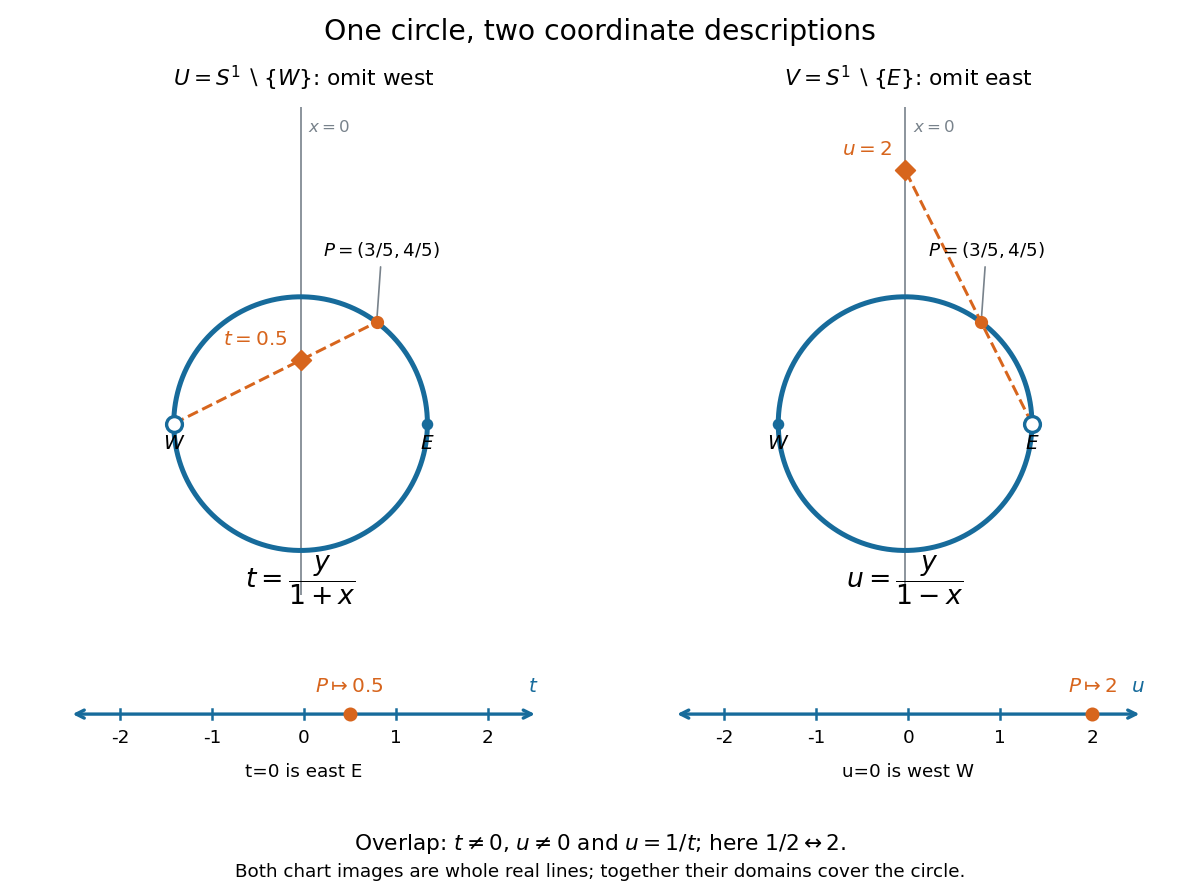
To verify the homeomorphisms, solve the displayed equations for $(x,y)$. The inverse functions areEach formula lies on the circle, avoids its excluded point, and is continuous for every real argument. Substitution into the projection formulas returns $t$ or $u$; substitution in the other direction returns $(x,y)$. Thus these are continuous bijections with continuous inverse functions, as required for coordinate charts. Since the Euclidean plane is Hausdorff and second countable, the subset $S^1$ with its subspace topology is too. This checks all three conditions for a topological manifold, rather than just drawing a smooth-looking curve.

On the overlap $U\cap V$, both $x=\pm 1$ are excluded, so $y\ne 0$. Using $y^2=1-x^2$, the topological transition map isFor example, $(x,y)=(3/5,4/5)$ has $t=1/2$ and $u=2$. The two connected components of the overlap, the upper and lower arcs, correspond to the positive and negative parts of the punctured real line. The values $t=0$ and $u=0$ represent $E$ and $W$, respectively, and belong to only one chart each. The reciprocal coordinate change and its inverse function are smooth functions away from zero, so this topological atlas also supplies a smooth atlas.

Why can neither chart be enlarged to a single coordinate chart on the whole circle? The circle is a closed set and a bounded set in the Euclidean plane, hence compact by the Heine-Borel theorem. A global coordinate chart would give a homeomorphism to a nonempty open set $O\subseteq \mathbb{R}$. Its image would be compact and therefore closed in the real line. By connectedness of the real line, this forces $O=\mathbb{R}$, which is not compact. This is the one-dimensional instance of no compact manifold has a single Euclidean chart. Locally the circle is indistinguishable from the real line; globally compactness obstructs a single chart.