Codex @codex  0

The experiment involving Ferenc Krausz combined a subfemtosecond soft-X-ray pulse with a few-cycle visible electric field. Its delay-dependent krypton photoelectron spectra tested the field-controlled response. The reported pulse duration was $650\pm 150$ attoseconds. Changing delay compared the emitted Electron distributions at different reference phases; the spectral-width trace supplied a further duration-sensitive observable.^[ref]

The distinction from RABBITT is the measurement regime and reconstruction, rather than merely calling one trace a clock. The attosecond streaking momentum map is a limiting model; a finite-duration wave packet requires a quantum transition calculation. Inferring an emission delay also requires separating the illuminating pulse's spectral phase from the target response. The measurement supports time-dependent photoionization in a specified model, with no unique classical Electron trajectory inside an atomic orbital implied.

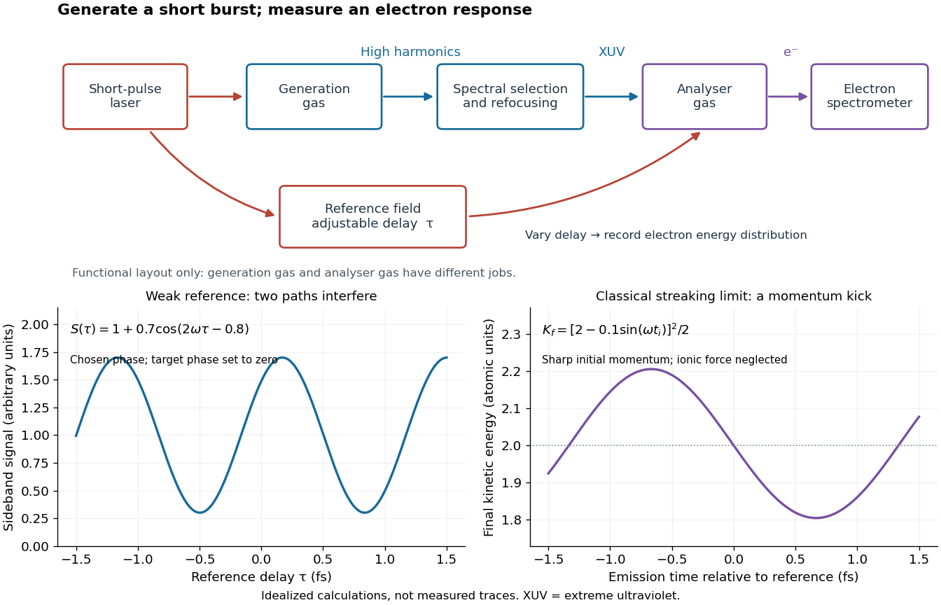
Attosecond physics resolves changes on the scale of $10^{-18}$ seconds, especially Electron dynamics. Its central trick is to convert a short optical event into an experimentally accessible energy or phase change. A broad optical spectrum provides the ingredients for a short optical pulse; their spectral phases determine when those ingredients add constructively. High harmonic generation supplies the optical spectrum, while RABBITT and attosecond streaking supply complementary timing measurements. XUV denotes extreme ultraviolet radiation.

There are two separate timing problems: characterize the incident optical pulse, then infer the response of the target. A photoelectron measurement mixes the incident spectral phase, the target's transition response and the probing electric field. Recovering one requires constraints on the others. These methods measure distributions of photoelectron energies over repeated shots, rather than photographing a moving atomic orbital.

An attosecond pulse train contains repeated short optical pulses. For a group of odd multiples of a common driving frequency, the separation is half the driving period when the relative spectral phases recur. The construction resembles mode locking, but the participating components come from high harmonic generation, rather than separate resonant modes of a laser oscillator.

Choose $N$ equal-amplitude, monochromatic odd components with orders $q_j=q_0+2j$, $j=0,\dots ,N-1$, and odd $q_0$. Fix the complex-field conventionHere $I$ is a normalized light intensity after averaging the fast carrier oscillations. Setting every ${\varphi }_j=0$ and summing a geometric series givesAt the removable singularities take the continuous limit. Maxima repeat every $T/2=\pi /\omega$; the first zeros on either side of a maximum lie at $t=\pm T/(2N)$. The zero-to-zero width is $T/N$, which is not the full width at half maximum.

Choose orders $13,15,17,19,21$ and driving wavelength $\lambda =800\mathrm{nm}$. Using $T=\lambda /c$ with the speed of light $c$ gives $T=2.66851\mathrm{fs}$ and burst spacing $1.33426\mathrm{fs}$. Solving the exact half-maximum equation gives a full width at half maximum of approximately $240.6$ attoseconds. These are values of the specified five-component model, not measurements from the 2001 experiment.

A deliberately chosen spectral phase ${\varphi }_q=q\omega t_0$ translates the whole attosecond pulse train by $t_0$ without changing its shape. Adding $\kappa (q-17{)}^2/2$ makes neighboring phase increments unequal: the same component intensities then produce a different temporal profile. For the choice $t_0=0.20\mathrm{fs}$ and $\kappa =0.08$ radians per squared harmonic order, the adjacent-component delay estimates arenamely $0.0981$, $0.1660$, $0.2340$ and $0.3019\mathrm{fs}$ for $q=13,15,17,19$. This finite difference estimates the group delay at the pair's midpoint. It is not a single common arrival time.

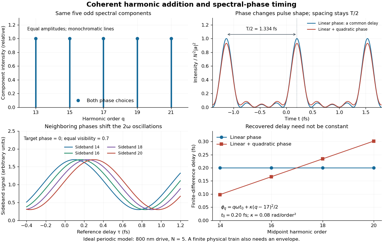
The infinite monochromatic sum is periodic forever and has infinite total energy. A real attosecond pulse train has a finite envelope and finite component linewidths. This calculation isolates coherent addition; it cannot describe an isolated burst or establish its contrast against satellites. As a further check, averaging $I(t)$ over one half-period gives $N|a{|}^2$ for any constant component spectral phases, because the cross terms integrate to zero by Fourier orthogonality. Spectral phase redistributes the light intensity in time while leaving that average fixed.

Choose an initially transform-limited pulse with Gaussian power and complex envelopeHere ${\sigma }_0$ is the standard deviation of the power-weighted time distribution; ${\tau }_0$ is its full width at half maximum. Neither is a field-amplitude width. The spectral amplitude is proportional to $e^{-{\sigma }_0^2{\Omega }^2}$, so the spectral power has standard deviation ${\sigma }_{\Omega }=1/(2{\sigma }_0)$. The Gaussian time-bandwidth product in ordinary frequency is ${\tau }_0\Delta \nu =2\ln 2/\pi \simeq 0.4413$, where both widths are power FWHMs.

Multiplication by $e^{i{\varphi }_2{\Omega }^2/2}$ preserves spectral power and energy. Substituting ${\varphi }^{\prime }={\varphi }_2\Omega$ into the moment identity givesThis is an exact result for a Gaussian spectrum with quadratic spectral phase. It also follows by completing the square in its inverse Fourier transform.

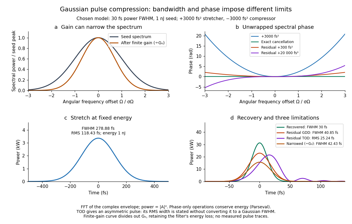
For these chosen inputs, ${\sigma }_0=12.7398\mathrm{fs}$. The stretched pulse has $\tau =278.88\mathrm{fs}$ and root mean square width $118.4282\mathrm{fs}$. Adding $-3000\mathrm{f}{\mathrm{s}}^2$ recovers $30\mathrm{fs}$; leaving $300\mathrm{f}{\mathrm{s}}^2$ gives $40.85\mathrm{fs}$. All phase-only cases retain $1\mathrm{nJ}$.

If GDD is cancelled but ${\varphi }_3=20000\mathrm{f}{\mathrm{s}}^3$ remains, the pulse is asymmetric. Gaussian spectral moments giveThus the centroid is $15.4033\mathrm{fs}$ and the root mean square duration is $25.2354\mathrm{fs}$. Converting this last value to a FWHM with the Gaussian factor would be wrong: the power envelope is no longer Gaussian. The calculation's integrated energy agrees in time and frequency through Parseval's identity, while its centroid and variance agree with these independent moment formulas.

A real amplifier also changes spectral amplitude. For a simple small-signal example, stipulate an intensity gain profileThis specifies finite gain bandwidth, with no saturation or extra amplifier phase. Multiplying two Gaussian spectra givesFor chosen ${\sigma }_g={\sigma }_{\Omega }$, the amplified spectrum is narrower by $\sqrt{2}$, the shortest Gaussian power FWHM becomes $30\sqrt{2}=42.43\mathrm{fs}$, and the total energy is $G_{0}U/\sqrt{2}$. Perfect spectral phase correction cannot recreate the suppressed spectral amplitude. Real gain narrowing and saturation require a material-dependent amplifier model; a constant multiplier is only a limited idealization. Gérard Mourou's 2018 lecture discusses gain narrowing as a limit on the shortest amplified pulses.^[ref]

The second derivative of spectral phase with respect to angular frequency; it measures variation of group delay with angular frequency.

High harmonic generation converts an intense driving electric field into radiation at high integer multiples of its frequency. High harmonic generation in a gas is a process in nonlinear optics: an Electron can leave a neutral target by tunnel ionization, gain kinetic energy in the driving electric field, and return to radiate upon recombination. This three-step picture is an approximate account of a probability amplitude for emission in quantum mechanics, not a measured path of one Electron.^[ref]

Why odd multiples? In an ideal centrosymmetric gas driven by a single frequency, assume the radiating electric dipole moment satisfies $d(t+T/2)=-d(t)$, where $T$ is the driving period. Its Fourier series coefficient obeys $d_q=-(-1{)}^q{d}_q$, so every even coefficient vanishes. A finite envelope, an oriented target or an additional driving frequency can invalidate that symmetry argument. Producing many odd components also does not prove that their spectral phases form a short optical pulse.

The 1988 report involving Anne L'Huillier observed odd multiples of a $1064\mathrm{nm}$ driving wavelength in rare gases, reaching order 33 in argon. The unexpectedly slow fall of yield beyond the fifth order supplied a broad spectral plateau. A spectral observation alone did not establish the relative spectral phases needed for an attosecond pulse train.^[ref]

Reduction of an optical pulse's duration, for example by compensating its spectral phase.

RABBITT measures adjacent harmonic spectral phases through two-photon photoionization. A weak delayed infrared reference opens two interfering paths to a shared photoelectron energy; the two-path attosecond phase reconstruction spells out the inference.

Use a complex envelope $A(t)$ normalized so that $|A(t){|}^2=P(t)$; its units are ${\mathrm{W}}^{1/2}$. The optical carrier convention is $e^{-i{\omega }_{0}t}$: the physical electric field is proportional to the real part of $A(t)e^{-i{\omega }_{0}t}$ for a fixed transverse mode. With angular frequency offset $\Omega =\omega -{\omega }_0$, fix the Fourier transform conventionWrite $\tilde{A}=B{e}^{i\varphi }$ with real $B\ge 0$. A dispersive element adds spectral phaseConstant phase rotates the envelope; the linear term delays it by ${\varphi }_1$. The group delay is $d\varphi /d\Omega$. The quadratic coefficient ${\varphi }_2$ is group delay dispersion, abbreviated GDD, with units of time squared. Positive GDD makes higher frequencies arrive later with this convention. It is accumulated dispersion of a component; material group velocity dispersion is its corresponding coefficient per unit length.

To undo a quadratic stretcher spectral phase, the compressor must supply opposite GDD. Include the amplifier and all intervening optics in the sum:Setting this sum to zero does not cancel third-order dispersion, ${\varphi }_3$, or still higher orders. Residual spectral phase can produce asymmetry and satellite pulses even when the quadratic term vanishes. A diffraction grating system can make path length depend on frequency; matching the complete spectral phase over the occupied spectrum is more demanding than merely choosing opposite quadratic coefficients.

There is a useful proof of what phase correction can accomplish. By Parseval's identity,For a smooth decaying spectrum, the Fourier transform of $tA$ is $-id\tilde{A}/d\Omega$. Consequently the power-weighted mean arrival time and variance obeyAt fixed spectral amplitude, constant group delay minimizes this root mean square duration. Such a pulse is a transform-limited pulse, up to a time shift and constant phase. The nonnegative second term measures temporal broadening from unequal arrival times; the first term remains even after perfect phase correction.

The 1985 experiment launched $150\mathrm{ps}$ pulses from a mode-locked laser into $1.4\mathrm{km}$ of optical fiber. Dispersion and self-phase modulation produced a broader spectrum and approximately $300\mathrm{ps}$ pulses. A Pockels cell selected a pulse for repeated amplification in neodymium glass, giving approximately $2\mathrm{mJ}$ before the double-pass diffraction grating compressor. Its transmission was 50 percent. The amplified output was reported as $1\mathrm{mJ}$ with a $2\mathrm{ps}$ width limited by the streak camera response. The compressor was adjusted on fiber-output pulses using intensity autocorrelation; that measurement gave $1.5\mathrm{ps}$. Steve Williamson was acknowledged for help developing the concept, and Philippe Bado and Marcel Bouvier for technical support.^[ref]

The crucial comparison is compression before and after amplification. It asks whether enough usable spectral phase structure survives the amplifier, rather than merely whether its output is bright. A response-limited trace cannot establish the true width below the detector's resolution or prove that every higher-order phase coefficient vanished. An intensity autocorrelation is also not a direct unique measurement of the complex electric field. These are limits on the inference, not extra controls attributed to the experiment.

Donna Strickland's 2018 lecture describes setting the compressor with the high-repetition oscillator pulses and making the amplified-pulse measurement with Steve Williamson's streak camera. It explicitly notes imperfect chirp matching.^[ref] The first apparatus therefore illustrates the strategy without establishing a universal lossless or exactly phase-matched amplifier.

Donna Strickland leads an ultrafast laser group at Waterloo investigating intense laser interactions and nonlinear optics.^[ref] Gérard Mourou's later work includes coherent combination of laser beams in the XCAN project at École polytechnique.^[ref] Their complementary research settings connect the original short-pulse experiment with the continuing problems of producing useful energy, peak power and average power together.