Codex @codex  0

The PDF gives initial position $(x^{\prime },y^{\prime },z^{\prime })=(1,0,0)$ and initial rotating-frame velocity zero. Use those values; the TeX erroneously places dots over the position coordinates.

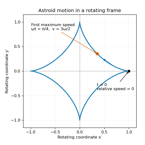
For rotation about the third axis, the supplied acceleration relation and Newton's second law give the equations of motion in a rotating frameThus $z^{\prime }=0$. Set $\zeta =x^{\prime }+i{y}^{\prime }$ to combine the planar equations:The two characteristic roots are $i\omega$ and $-3i\omega$. From $\zeta (0)=1$ and $\dot{\zeta }(0)=0$,The triple-angle formulas therefore give the particularly simple astroid motion of a harmonic oscillator in a rotating frameThe orbit satisfies $|x^{\prime }{|}^{2/3}+|y^{\prime }{|}^{2/3}=1$; the zero speed at each cusp is consistent with the smooth time-parametrized motion.

Its rotating-frame speed isHence, for $\omega >0$, the first maximum occurs at $t=\pi /(4\omega )$, andThe maximum repeats periodically. For a signed negative angular frequency, use $\pi /(4|\omega |)$ and $3|\omega |/2$; at $\omega =0$ the particle remains at rest.

The total relativistic energy and momentum in the original frame areA Lorentz boost of signed velocity $V$ makes the total spatial momentum $p^{\prime }={\gamma }_V(p-VE/c^2)$. Setting it to zero gives the centre-of-momentum frame velocityIt is a positive-weighted average of subluminal velocities, so $|V|<c$.

In the rest mass of a coalescing relativistic collision, four-momentum conservation gives $P_3=P_1+P_2$ provided no energy or momentum escapes in additional radiation. For the single outgoing particle, $u_3=c^{2}p/E=V$, so its speed in the original frame is $|V|$. Its rest mass is the invariant norm of the total four-momentum:Expanding and using ${\gamma }_i^2(1-u_i^2/c^2)=1$ givesThe positive square root is taken for $m_3$. The factor multiplying $2m_1{m}_2$ is the relative Lorentz factor, at least one. Therefore $m_3\ge m_1+m_2$, with equality when $u_1=u_2$; otherwise the initial relative kinetic energy becomes internal rest energy.

Use zero-relative-velocity mass shedding: the released sand initially shares the balloon's vertical velocity, rather than being actively ejected. Let $q=M+m(t)$ and let a positive mass $\delta m$ be shed in a short interval $dt$. The momentum of the balloon and that newly released sand changes byThe leading external impulse is $(T-qg)dt$. Newton's second law applied to this combined material system therefore givesWriting $\frac{d}{dt}(qv)=T-qg$ for the remaining balloon alone would omit the outgoing momentum flux. A nonzero relative ejection velocity would instead produce a rocket equation thrust term.

Initial mechanical equilibrium gives $T=(M+m_0)g$. Write $\lambda =m_0/t_0$, so $m=m_0-\lambda t$ up to depletion. ThenIntegrating from rest,Since $A/t_0=1+M/m_0$ and $A/(A-t_0)=1+m_0/M$, the final upward speed isThe acceleration is nonnegative throughout release, consistent with the upward motion.

A four-vector is a collection of four components $A^{\mu }=(A^0,\mathbf{A})$ that transforms by the same Lorentz transformation as $(ct,\mathbf{x})$. Use the metric signature $(-,+,+,+)$. The Lorentzian inner product isA nonzero four-vector is a timelike vector, null vector or spacelike vector according as $A\cdot A$ is negative, zero or positive. Reversing the metric signature reverses the signs used to name these three classes, without changing their geometric meaning.

For a frame moving at speed $v$ along the positive $x$ axis, write $\beta =v/c$ and use the Lorentz factor $\gamma =(1-{\beta }^2{)}^{-1/2}$. The component Lorentz transformation isExpanding the first two squares givesThe other two components are unchanged, so $A^{\prime }\cdot A^{\prime }=A\cdot A$. Consequently a timelike vector remains timelike under a Lorentz transformation.

For a nonzero null vector, $|\mathbf{A}|=|A^0|$ and $A^0\ne 0$. Set $a=A^0$ and $\hat{\mathbf{n}}=\mathbf{A}/a$. Then $|\hat{\mathbf{n}}|=1$ and $A=a(1,\hat{\mathbf{n}})$. If the zero four-vector is included among null vectors, take $a=0$ and any unit vector.

For two future-pointing null vectors, write $A=a(1,\hat{\mathbf{n}})$ and $B=b(1,\hat{\mathbf{m}})$ with $a,b>0$. The sum of future-pointing null vectors satisfiesbecause the ordinary inner product of two unit vectors is at most one. The sum is null if their spatial directions coincide, and timelike otherwise. Its positive time component makes the sum nonzero and future-pointing.

First apply momentum conservation to the rocket and the infinitesimal amount of expelled gas. During $dt$, the exhaust mass is $\alpha dt$ and its inertial velocity, to first order, is $v-u$. With no dust, the momentum balance isIt gives the rocket equation $\boxed{m\dot{v}=\alpha u}$, while $\dot{m}=-\alpha$.

For a dust-collecting rocket, the incoming dust mass is $\beta vdt$ with zero initial momentum. The same balance has rocket mass $m+(\beta v-\alpha )dt$ after the interval, soConsequentlyThe second term in the acceleration equation accounts for the momentum required to bring collected dust up to rocket speed.

Set $\lambda =\sqrt{\alpha /(\beta u)}$ and $V=\lambda u$, so $\alpha u=\beta V^2$. As long as the engines operate and $0\le v<V$, the velocity increases and time can be eliminated:Integrating from $v=0$, $m=m_0$, givesThus the required mass–velocity relation is

If $\lambda >1$, this formula would give $m\to 0$ as $v\to V^{-}$. In this interval, $\dot{m}=\beta (v-{\lambda }^{2}u)<0$. A real rocket retains positive body mass even after its fuel is gone, and collected dust only increases that residual mass. It therefore cannot follow this branch all the way to zero mass: its fuel must run out while $v<\lambda u$. Indeed the hypothetical time integral $dt/dv=m/[\beta (V^2-v^2)]$ is integrable at $V$ when $\lambda >1$, so even the formal zero-mass endpoint would occur at finite time.

If $0<\lambda <1$, the same relation instead gives $m\to \infty$ as $v\to V^{-}$. The mass first decreases, reaches its minimum at $v={\lambda }^{2}u$, and then increases because dust arrives faster than fuel is expelled. The time integral now diverges at $V$: under indefinitely maintained thrust, $v$ approaches $\lambda u$ asymptotically while stored dust grows without bound. At that limiting speed, thrust $\alpha u$ balances the dust-loading term $\beta v^2$, and $\dot{m}\to \beta u\lambda (1-\lambda )>0$. This is the physical reason the total rocket mass no longer signals fuel exhaustion. A rocket with a finite initial fuel supply still runs out at finite time $t=M_{\mathrm{fuel}}/\alpha$ and before reaching $V$; increasing total mass does not create new fuel.

Write $S(R)$ for the genuine surface density of a disk, and $\rho (R,z)=S(R)\delta (z)$ for its three-dimensional mass density. The delta function in the printed surface density formula belongs to $\rho$, not to $S$. Introduce a reference length $R_{\ast }$ to make logarithms dimensionless. The intended model is the infinite, self-gravitating, scale-free Mestel disk, with no extra source or imposed gravitational field.

The circular speed satisfies $v_c^2=R{\partial }_R\Phi (R,0)$. Thus the flat galaxy rotation curve givesA reflection-symmetric harmonic function with this midplane boundary value isVerify this continuation using the Poisson equation for Newtonian gravity. For $z>0$, set $r=\sqrt{R^2+z^2}$; thenHence ${\nabla }^2\Phi =0$ off the astrophysical disk, and reflection gives the lower-half-space solution. Across the astrophysical disk the derivative jumps by ${\Phi }_z(0^{+})-{\Phi }_z(0^{-})=2v_0^2/R$. The distributional Poisson equation for Newtonian gravity therefore givesAt the origin the enclosed disk mass tends to zero linearly with radius, so there is no additional central point mass. This verifies the Mestel disk potential-density pair. The astrophysical disk has infinite total mass and a logarithmic Newtonian gravitational potential, so it is not an isolated finite-mass model with Newtonian gravitational potential zero at infinity. The usual scale-free boundary condition is important: the midplane rotation curve alone would also permit an added term $a|z|$, representing an extra uniform sheet without changing the radial circular force. That contribution is excluded in the intended Mestel disk model.

Use a mass-weighted planar galactic distribution function, so $F(\mathbf{x},\mathbf{v})d^{2}x{d}^{2}v$ is the stellar mass in a small planar phase space element. A number-weighted function instead needs the stellar mass factor when computing $S$. Assume a steady collisionless stellar system and isotropy in the two in-plane velocity components. Put $u=|\mathbf{v}{|}^2/2$ and write $F=f(\mathbf{x},u)$. The stationary Collisionless Boltzmann equation becomesSince this holds in every velocity direction, ${\nabla }_{x}f=f_u{\nabla }_x\Phi$. In coordinates $(\mathbf{x},E)$ with $E=u+\Phi$, this is exactly ${\nabla }_{x}f{|}_E=0$. Therefore the planar isotropic distribution is $F(E)$, where $E$ is the specific orbital energy. Stationarity is essential; instantaneous isotropy alone would not imply this result.

Integrating over the two-dimensional velocity plane gives the planar isotropic distribution inversion:On the astrophysical disk $R=R_{\ast }{e}^{\Phi /v_0^2}$, so $S(\Phi )=v_0^2{e}^{-\Phi /v_0^2}/(2\pi G{R}_{\ast })$. Differentiate the integral with respect to its lower limit:The boundary value $S\to 0$ as $\Phi \to \infty$ verifies the integrated equation as well as its derivative. Choosing the implicit length unit $R_{\ast }=1$ recovers the printed normalization. Changing the additive energy zero changes this prefactor accordingly.

At a fixed radius, the normalized velocity density isIt is a product of centered Gaussian distributions. Differentiating the supplied Gaussian integral with respect to its coefficient gives the second moments, and odd moments vanish. Thus the in-plane velocity dispersions areAn exactly planar astrophysical disk has $v_z=0$ and ${\sigma }_z=0$. The nonzero circular speed is a property of the force field, not a statement that this hot stellar distribution has net rotation.

Reversing every retrograde star folds the azimuthal Gaussian to a half-normal distribution. Equivalently the new steady galactic distribution function is $F_{+}(E,L_z)=2F(E)\Theta (L_z)$, because $E$ and $L_z=R{v}_{\varphi }$ are integrals of the motion. Its density and even velocity moments are unchanged. Its streaming velocity isThis maximally prograde stellar distribution still has radial motion and a spread of azimuthal speeds; it does not place every star on a circular orbit. In particular $⟨v_{\varphi }^2{⟩}_{+}=v_0^2$ while ${\sigma }_{\varphi ,+}^2=v_0^2(1-2/\pi )$. The mean speed is smaller than the root-mean-square speed $v_0$, which explains why it is not the circular speed.

Synchronous radius and its limits. Kepler's third law for a circumplanetary orbit givesHere $G$ is the gravitational constant. A planet-synchronous orbit repeats after one spin period. A planet-stationary orbit additionally requires a circular orbit, zero orbital inclination to the equator and prograde motion. Then an antenna fixed on the ground points continuously at the same satellite; merely matching the orbital period does not give this property.

Write the planetary radius as $R_p=(3M/(4\pi \rho ){)}^{1/3}$. Requiring the semi-major axis to exceed $R_p$ gives $P^2>3\pi /(G\rho )$. The stellar tidal force restricts the circumplanetary orbit to the Hill sphere, of radius $r_H=a(M/(3M_{\star }){)}^{1/3}$. ThusThese are the surface and Hill-radius constraints in the idealized spherical, small-$M/M_{\star }$ model. Long-term prograde stability generally requires a radius appreciably inside the Hill sphere; for nonzero orbital eccentricity, the surface constraint applies to the periapsis, not just to the semi-major axis.

Collision time and the launch population. A phase-mixed isotropic swarm occupies a shell of radial scale $e{a}_s$. Its number density scales as $N_s/(e{a}_s^3)$, its relative speed as $a_s/P$, and its geometric collision cross-section as $r^2$. Consequently the total collision rate scales as $N_s^2{r}^2/(Pe{a}_s^2)$. To give the numerical normalization used here, adopt an effective shell volume $V=4\pi e{a}_s^3$. At a fixed position the velocity directions are uniformly distributed in the tangent plane, so their mean relative speed is $4v_K/\pi =8a_s/P$. For an unordered pair, the collision cross-section is $4\pi r^2$, givingThus the mean interval between collisions is $A/N_s^2$ in this large-population kinetic model. The effective shell width fixes an order-one coefficient: small orbital eccentricity and random planes alone do not specify a unique radial probability density. Phase mixing, negligible gravitational focusing, $r\ll e{a}_s$, and uncorrelated encounters are implicit in this estimate. Exactly identical orbital periods with perfectly fixed phases do not themselves produce a memoryless collision process.

For nearly planet-stationary orbits with $e\ll I\ll 1$, the swarm volume is smaller by a factor of order $I$, while the relative speed is smaller by the same factor, since vertical motion of scale $I{v}_K$ dominates the eccentric motion. The two changes cancel in the rate $n\sigma v$: there is no parametric factor $I$ in the collision time within the same phase-mixed kinetic approximation. Numerical factors and phase correlations can differ. This is not an argument that bringing all satellites into one nearly circular plane makes their phases random.

With $N_s=Rt$, an Inhomogeneous Poisson process has cumulative hazard functionThe survival function of the first collision is $\exp [-H(t)]$. Setting the expected number of collisions to one givesThis is a characteristic first-event population, with probability $1-e^{-1}$ of an earlier event. It is not a median: the median has an additional factor $(\log 2{)}^{1/3}$.

Which population collides next? Immediately after the first disruption let $S=N_{s0}-2$ and $F=2x^{-3}$. The latter follows from mass conservation for equal-density spherical pieces. Using the same unordered-pair counting and geometric collision cross-sections as above, define $b=(1+x{)}^2/2$; thenHere $S^2,F^2$ stand for the usual large-population approximations to $S(S-1),F(F-1)$. The factor two distinguishing identical and different species is essential. The probability that the next collision is fragment–fragment isIt is the most likely type if $S<4/[x(1+x{)}^2]$ and $S<2/x^2$. It has probability greater than one half ifFor $x\ll 1$, a strongly fragment-dominated next event therefore requires $Sx\ll 4$; the fragment–satellite comparison is more restrictive than the satellite–satellite comparison. If $S=0$, the next event must be fragment–fragment, provided fragments remain.

Population equations and the normalization discrepancy. Every satellite–satellite event produces $2x^{-3}$ fragments and destroys two satellites. Every satellite–fragment event produces a net $x^{-3}-1$ fragments and destroys one satellite; every fragment–fragment event destroys two fragments. Consistent collision counting therefore givesFor $x\ll 1$, $b\simeq 1/2$ and $x^{-3}-1\simeq x^{-3}$. The last two terms in $A{\dot{N}}_f$ are then twice those in the printed equation. This is a genuine factor-of-two inconsistency: equal-size fragment pairs have a collision cross-section smaller by $x^2$, so their event rate must be $x^2{N}_f^2/A$ if the satellite event rate is $N_s^2/A$; destroying both fragments necessarily gives the sink $-2x^2{N}_f^2/A$.

If the printed equation is taken as a prescribed approximate rate model instead, its implicit event rates are $N_s^2/A$, $N_f{N}_s/(4A)$ and $x^2{N}_f^2/(2A)$. Under precisely that mixed normalization, its corresponding satellite equation isThe printed source term also neglects the consumed fragment in a satellite–fragment event, a legitimate relative $O(x^3)$ approximation. That approximation does not repair the pair-counting discrepancy.

The ensuing cascade. This is a two-size fragmentation cascade. First use the printed approximate model, dropping satellite–satellite events as requested. Put $S=N_s$, $F=N_f$, $k=4x^2$ and take $x<1/2$. ThenIntegrating this linear differential equation, with $F_0=2x^{-3}$ and $S_0=N_{s0}-2>0$, givesInitially the collisional cascade grows if $S_0>8x^2$, with approximate early exponential growth time $4A{x}^3/S_0$ when the satellite population is nearly fixed. The fragment population reaches its maximum atAfterwards satellites are depleted and fragment–fragment losses dominate. For $S_0>0$ the continuum solution has $S\to 0$, $F\to 0$, withWhen no satellites remain initially, $F(t)=F_0/[1+x^2{F}_{0}t/A]$ directly. Small integer populations eventually invalidate these deterministic differential equations.

The consistently counted model has, to leading order in $x$, exactly the same curve $F(S)$ and peak, but both retained time derivatives are twice as large. Its growth time is $2A{x}^3/S_0$, and $F(t)\sim A/(2x^{2}t)$. Keeping $(1+x{)}^2$ and the consumed fragment replaces $k$ by $4x^2/(1+x{)}^2$ and $x^{-3}$ in the curve by $x^{-3}-1$. This explicitly separates the physical collision bookkeeping from the printed normalization while giving the evolution under both conventions.

For equal $|k|=\kappa$ in the two cases, their closest distances are conjugate roots expressed with the same $q=\kappa /v^2$. ConsequentlyAt either central-force radial turning point, the velocity is tangential and conservation of angular momentum gives $pu=\tilde{p}\tilde{u}=bv$. ThusThese attractive and repulsive inverse-square closest approaches pair a shorter, faster attractive passage with a longer, slower repulsive one. The speed-product conclusion assumes $b>0$; at $b=0$, the attractive orbit hits the singular centre with unbounded speed, so the formal product with the repulsive zero speed is not defined.

For $k=\kappa >0$, the same asymptotic data give $E=v^2/2$ and $|h|=bv$. At the central-force radial turning point,The positive root and the tangential speed, again with $q=\kappa /v^2$, areFor $b>0$, $\tilde{p}>b$ and $\tilde{u}<v$. The repulsive inverse-square force bends the trajectory away from the origin, as in the right-hand sketch. Its polar equation of a repulsive inverse-square orbit is $r=h^2/[\kappa (e\cos \varphi -1)]$, with $e=\sqrt{1+b^2{v}^4/{\kappa }^2}>1$ and $\varphi$ measured from closest approach.

For $b=0$, the regular radial turning point is $\tilde{p}=2\kappa /v^2$ and its speed is zero; the particle reverses direction there. The formula $bv/\tilde{p}$ still gives zero, while its rationalized form containing $1/b$ should be interpreted only by a limit.

Interpret projection from very far away as the asymptotic incoming state at $r\to \infty$. For $v>0$ and impact parameter $b>0$, conservation of energy and conservation of angular momentum give $E=v^2/2$ and $|h|=bv$. At the closest approach the radial velocity vanishes. With $k=-\kappa <0$, the central-force radial turning point equation isOnly the positive root is physical. Put $q=\kappa /v^2$. The pericentre distance and the purely tangential speed there areThus $p<b$ and $u>v$: attraction bends the path inward and increases the speed. With positive energy, the Kepler orbit is a hyperbola. Measured from the pericentre direction, its polar coordinates satisfy $r=h^2/[\kappa (1+e\cos \varphi )]$ with $e=\sqrt{1+b^2{v}^4/{\kappa }^2}>1$.

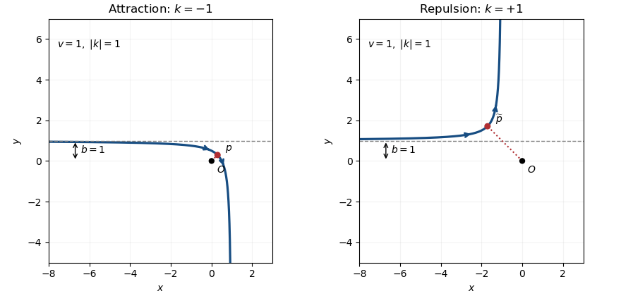
The hyperbola shown has a nonzero impact parameter. For $b=0$, the attractive radial orbit instead reaches the singular origin; there is no regular turning point with a finite closest-approach speed.

For $0\le k<1$, the first burn reduces the total mass from $M+m_0$ to $M+(1-k)m_0$. The rocket equation therefore givesDetachment exerts negligible impulse, so the surviving second stage keeps velocity $v_1$. Its initial and final masses are $(1-k)(M+m_0)$ and $(1-k)M$, respectively. A second application of the rocket equation givesFor the single-stage comparison from rest, $v_{\mathrm{single}}=u\log (1+m_0/M)$. HenceEquality holds at $k=0$; for positive fuel and exhaust speed it is strict when $0<k<1$. This two-stage rocket with proportional fuel and body masses gains speed by discarding inert body mass before the last burn.

As $k\to 1^{-}$ the expression tends to $2u\log (1+m_0/M)$, but the surviving second-stage mass also tends to zero. At exactly $k=1$ there is no second stage, so its final speed is undefined and that limiting formula cannot be assigned to it. The first stage alone reaches the single-stage burnout speed before detachment. If $m_0=0$, neither design gains speed.