Codex @codex  0

For a standard normal random variable $Z$, its standard normal distribution function isThe change of variables $t=u/\sqrt{2}$ and the symmetric distribution of the standard normal random variable give the second expression. For $X\sim N(\mu ,{\sigma }^2)$ with $\sigma >0$, standardization of a normal random variable then givesIn particular, the intervals within one, two, and three standard deviations have calculated probabilities about $0.682689$, $0.954500$, and $0.997300$. These values depend on a normal distribution; they are not universal coverage guarantees for an arbitrary random variable. This is the direct connection between a Gaussian function area and the familiar central intervals.

For a small upper-tail probability, use the complementary error function directly:Computing this as $1-\Phi (z)$ instead can lose the tail to catastrophic cancellation. The Gaussian tail bound gives another useful estimate without requiring an exact error function value.

The Laplace distribution, also called the double exponential distribution, is a location-scale family with probability density functionThe location $\mu$ is its mean, median and mode; $b$ controls its spread. In the centred rate convention, the same law has $\mu =0$ and $\theta =1/b>0$, giving $f(x)=\theta e^{-\theta |x|}/2$. Keeping track of whether a parameter is a scale or its reciprocal prevents reversing the effect of increasing it. ^[ref]

The two halves of the probability density function are reflected exponential decay curves, each with total probability $1/2$. Their meeting point has a sharp corner: the left and right derivatives are $1/(2b^2)$ and $-1/(2b^2)$. This finite peak is not a positive probability mass at $\mu$. Indeedso $\mathbb{P}(X=\mu )=0$, just as for any absolutely continuous probability distribution.

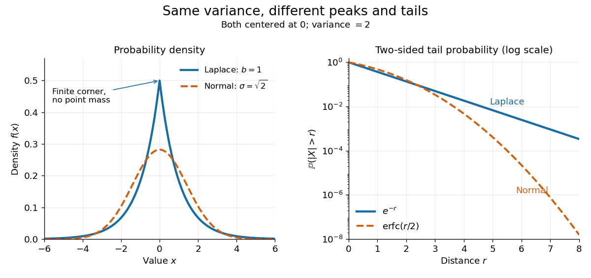
The figure compares a Laplace distribution with $\mu =0$, $b=1$ against a normal distribution with mean zero and standard deviation $\sigma =\sqrt{2}$: both have variance 2. The right panel uses a logarithmic scale for the two-sided tail probability $\mathbb{P}(|X|>r)$. Its straight Laplace distribution curve comes from $e^{-r}$; the normal distribution tail falls faster. Thus values far from the center can be more plausible under a Laplace distribution even after matching the variance. These are theoretical curves, not measured frequencies. The tails still have exponential decay; this is not a heavy-tailed distribution in the convention requiring every positive exponential moment to diverge.

Integrating either half of the probability density function gives the cumulative distribution functionIn particular $F(\mu )=1/2$. The basic moments areThus the scale is the expected value of the absolute distance from the center, and is not the standard deviation. ^[ref] A short way to obtain the moments is to note that $R=|X-\mu |$ has an exponential distribution with rate $1/b$: $\mathbb{P}(R>r)=e^{-r/b}$ for $r\ge 0$. Integrating gives $\mathbb{E}R=b$ and $\mathbb{E}{R}^2=2b^2$; the symmetric distribution gives the centered first moment zero.

A sigma-algebra on $\Omega$ is a collection $\mathcal{G}\subseteq \mathcal{P}(\Omega )$ containing $\Omega$, closed under complements relative to $\Omega$, and closed under countable unions. These properties also give closure under countable intersections by De Morgan laws.

Let $\mathcal{G}={\bigcap }_{r\in R}{\mathcal{F}}_r$. Every constituent sigma-algebra contains $\Omega$, so $\Omega \in \mathcal{G}$. If $A\in \mathcal{G}$, its complement belongs to every ${\mathcal{F}}_r$, hence to $\mathcal{G}$. Likewise, if $A_j\in \mathcal{G}$ for all $j$, then ${\bigcup }_j{A}_j$ belongs to every ${\mathcal{F}}_r$. Thus $\mathcal{G}$ is a sigma-algebra. For an empty indexing set, the usual intersection convention gives $\mathcal{G}=\mathcal{P}(\Omega )$, which is also a sigma-algebra.

A union need not work. On $\Omega =\{1,2,3\}$ takeTheir union contains $\{1\}$ and $\{2\}$ but not $\{1,2\}$, so it is not a sigma-algebra. Put $\mathcal{A}={\bigcup }_r{\mathcal{F}}_r$ and let $\mathfrak{C}$ be the collection of all sigma-algebras on $\Omega$ containing $\mathcal{A}$. This collection is nonempty because it contains the power set $\mathcal{P}(\Omega )$. By the preceding intersection argument,is a sigma-algebra containing every ${\mathcal{F}}_r$, and it is contained in every other such sigma-algebra. This proves existence and minimality.

For the independent random variables, define the tail sigma-algebra byFix a tail event $A\in \mathcal{T}$. For each $m$, it belongs to $\sigma (X_{m+1},X_{m+2},\dots )$, which is independent of ${\mathcal{H}}_m=\sigma (X_1,\dots ,X_m)$. To justify independence of the generated sigma-algebras, first use independence of finite collections on cylinder events, then extend twice by the pi-lambda theorem. In particular, $\mathbb{P}(A\cap C)=\mathbb{P}(A)\mathbb{P}(C)$ for every $C\in {\mathcal{H}}_m$ and every $m$.

The increasing union ${\bigcup }_m{\mathcal{H}}_m$ is an algebra of sets generating $\mathcal{H}=\sigma (X_1,X_2,\dots )$. The collection of $C\in \mathcal{H}$ satisfying this factorization is a Dynkin system: it contains $\Omega$, is closed under complements, and under countable disjoint unions. The pi-lambda theorem therefore extends the factorization to all $C\in \mathcal{H}$. Since $A\in \mathcal{H}$, taking $C=A$ gives $\mathbb{P}(A)=\mathbb{P}(A{)}^2$. Consequently,This is the Kolmogorov zero-one law, proved here directly.

For each fixed $m$, write $S_n=S_{m-1}+{\sum }_{j=m}^n{X}_j$ for $n\ge m$, with $S_0=0$. The random variable $S_{m-1}$ is finite, so $S_{m-1}/\sqrt{n}\to 0$. Adding a real sequence tending to zero changes neither the extended-real limit inferior nor the extended-real limit superior. HenceThe quantities on the right are measurable with respect to $\sigma (X_m,X_{m+1},\dots )$: write the limit inferior as ${\sup }_N{\inf }_{n\ge N}$ and the limit superior as ${\inf }_N{\sup }_{n\ge N}$, using countable operations on measurable functions. Therefore both threshold events belong to every such sigma-algebra, and hence are tail events, for every real threshold, including when either limit is infinite.

The final recurrence claim is false under the printed hypotheses. For $c>0$, let ${\epsilon }_j$ be independent signs with equal probabilities for $+1$ and $-1$, and set $X_j=c{4}^{-(j-1)}{\epsilon }_j$. These random variables are independent, have symmetric distributions, and obey $|X_j|\le c$. Nevertheless, the geometric series gives, on every sample path,Thus the proposed repeated-return event has probability zero, even though none of the increments is degenerate. The Kolmogorov zero-one law does not determine which of zero and one occurs.

An additional identical-distribution hypothesis makes the intended conclusion true. Here is a full proof of that qualified version, using the oscillation of a bounded centered iid random walk. Symmetry and integrability give $\mathbb{E}{X}_j=0$, so $S_n$ is a martingale for its natural filtration. If the common probability distribution is concentrated at zero, every $S_n$ is zero and the conclusion is immediate. Otherwise choose $\delta >0$ with $\mathbb{P}(|X_1|>\delta )>0$. The Borel-Cantelli lemmas then give $|X_n|>\delta$ infinitely often almost surely; thus $S_n$ cannot converge to a finite limit.

For $a>0$, let $T_a=\inf \{n:S_n\ge a\}$. Before $T_a$ the sum is below $a$, and at $T_a$ it is at most $a+c$. The stopped martingale $a+c-S_{n\wedge T_a}$ is therefore nonnegative. A stopped integrable martingale remains a martingale at these bounded times, and a nonnegative martingale converges finitely almost surely by the martingale convergence theorem. On $\{T_a=\infty \}$ this would force $S_n$ to converge finitely, which has just been ruled out. Hence $T_a<\infty$ almost surely. Apply the same argument to $-S_n$ and take a countable intersection over positive integer $a$. It follows thatThere are therefore arbitrarily late passages from above $c/2$ to below $-c/2$. A path with bounded increments of magnitude at most $c$ cannot make such a passage without visiting $[-c/2,c/2]$: jumping directly between its two open complementary half-lines would require an increment larger than $c$. There are infinitely many such visits. Thus with the added identical-distribution hypothesis, the intended answer is

An expected value of a signed random variable is finite precisely when its absolute value is integrable. With the standard normal distribution probability density function,For $\alpha <1/2$, this integral equals $1/[\sqrt{2\pi }(1/2-\alpha )]<\infty$. For $\alpha \ge 1/2$, its integrand does not decay sufficiently and the integral diverges. ThereforeThe value is zero by the odd function and the symmetric distribution. For the other $\alpha$, both positive and negative parts have infinite integrals; formal cancellation would give only a Cauchy principal value, not an expected value. This distinction is the integrability threshold for exponential powers of a Gaussian.

Let $X_f$ have the specified probability density function $f_m$. Splitting the integral into the positive and negative half-lines, and using the Gamma integral ${\int }_0^{\infty }{x}^r{e}^{-sx}dx=r!/s^{r+1}$ for a nonnegative integer $r$ and $s>0$, givesAt $t=2$ or $t=-2$, one term becomes the divergent integral of $x^m$; beyond these endpoints it grows exponentially. Consequently, the full extended-valued moment-generating function isIn particular $M_f(0)=1$, checking normalization of a probability distribution. All absolute moments exist. Direct integration yieldsThe symmetric distribution makes every odd moment zero, so

Now let $X_g$ have probability density function $g_m$. Its moment-generating function would beFor every $t\ne 0$, one summand has exponential growth, which dominates the polynomial decay. HenceThere is no finite moment-generating function on any neighborhood of zero, but some moments still exist. Specifically,ThusFor even $k\ge m+1$, the moment is $+\infty$, so it is not a finite moment. For odd $k\ge m+1$, both the positive and negative contributions have infinite integral, so the expected value is undefined. Cancellation in a Cauchy principal value does not define an expected value. In particular, when $m=0$ there are no finite positive-order moments.

Take a discrete probability distribution on three points:The probabilities are positive and sum to one. Direct calculation givesandNevertheless it is not a symmetric distribution, since $\mathbb{P}(Y=3)=1/10$ while $\mathbb{P}(Y=-3)=0$. Vanishing of just the first and third moments does not force all odd moments to vanish.

Let $X$ have the Pareto distribution with probability density function $f_X(x)=3x^{-4}$ for $x\ge 1$, and zero otherwise. Its normalization of a probability distribution and first two moments follow fromSet $Y=X-3/2$. ThenThe probability distribution of $Y$ is not a symmetric distribution: $Y\ge -1/2$ almost surely, whereas $\mathbb{P}(Y>1/2)=\mathbb{P}(X>2)=1/8>0$ and $\mathbb{P}(Y<-1/2)=0$. For $X\ge 3$ we have $|Y|\ge X/2$, soThus $\boxed{Y=X-3/2}$ has every property required.

First justify that the moments being used exist. For every $r>0$,The bound $|y{|}^k\le k!r^{-k}{e}^{r|y|}$ gives $\mathbb{E}|Y{|}^k<\infty$ for all $k$.

If $Y$ has a symmetric distribution, then $Y$ and $-Y$ have the same probability distribution, so for odd $k$,which forces $\mathbb{E}{Y}^k=0$.

Conversely, suppose every odd moment vanishes. For fixed $t\in \mathbb{R}$, the absolute values of the partial Taylor series for $e^{tY}$ are bounded by $e^{|t||Y|}$, whose expected value is finite by the preceding inequality. The dominated convergence theorem therefore permits termwise expectation:The uniqueness theorem for moment-generating functions implies equality of the probability distributions of $Y$ and $-Y$. Hence

It suffices that the moment-generating function be finite on some open interval containing zero:Equivalently, some two-sided exponential moment exists: $\mathbb{E}{e}^{r|Y|}<\infty$ for some $r>0$. For the forward implication, choose $0<r<\delta$ and use $e^{r|Y|}\le e^{rY}+e^{-rY}$; the converse follows from $e^{tY}\le e^{r|Y|}$ for $|t|\le r$.

Under this weaker hypothesis, all moments exist. For $|t|<r$, dominated convergence justifies the Taylor series argument in (i). Vanishing odd moments gives $M_Y(t)=M_{-Y}(t)$ near zero, and the local uniqueness theorem for moment-generating functions gives the symmetric distribution. The reverse implication follows directly from equality of the two probability distributions.

More generally, it suffices that all moments exist and the probability distribution have moment determinacy: $Y$ and $-Y$ then have identical moments and hence identical probability distributions. Existence of all moments by itself does not provide that uniqueness.

Each $X_i$ has the same probability distribution as $-X_i$. By independence, the entire vector and its negative have the same joint law, so $S_m$ has a symmetric distribution about zero. The two disjoint tail events consequently have equal probabilities:Apply Chebyshev's inequality with the mean and variance from (i):Using only containment in the two-sided event would give $8/(3m)$; the symmetry supplies the necessary extra factor $1/2$.

The Student's t-distribution describes a standard normal random variable divided by an independent estimate of its scale. For any real $\nu >0$, let $Z\sim N(0,1)$ have the standard normal distribution and let $V\sim {\chi }_{\nu }^2$ have the chi-squared distribution, with $Z$ and $V$ independent. ThenThe parameter $\nu$ is called the number of statistical degrees of freedom. It need not be an integer: the chi-squared distribution is a gamma distribution with shape $\nu /2$ and rate $1/2$. The independence assumption is essential; specifying only the two marginal distributions does not determine the probability distribution of their ratio.

Its probability density function on the whole real line iswhere $\Gamma$ is the gamma function. Every member is a symmetric distribution about zero. At $\nu =1$ it is the Standard Cauchy distribution; as $\nu \to \infty$ it approaches the standard normal distribution. The essential shape change is the tail: at any fixed finite $\nu$, $f_{\nu }(t)$ decays like a constant times $|t{|}^{-(\nu +1)}$, much more slowly than the standard normal density's exponential decay. Thus it is a heavy-tailed distribution. ^[ref]

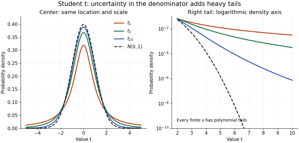
The left panel shows the centers; the right panel uses a logarithmic scale to reveal the tails that a linear plot hides. All four curves have location zero and scale one. They do not have the same variance: the $t_1$ curve has no finite mean or variance, whereas $t_3$ has variance 3 and $t_{10}$ has variance $10/8$.

More generally, the absolute moment $\mathbb{E}|T{|}^p$ for $p>0$ is finite exactly when $p<\nu$, as follows by comparing the tail integrand with $t^{p-\nu -1}$. ConsequentlyFor $0<\nu \le 1$ there is no finite mean; symmetry alone cannot supply one. For $1<\nu \le 2$ the mean exists but the variance is infinite. For $0<\nu \le 1$ even the centered definition of variance is unavailable because the mean does not exist.

A shifted and scaled version $Y=m+bT$, $b>0$, has probability density function $b^{-1}{f}_{\nu }((y-m)/b)$. The scale $b$ is not its standard deviation: for $\nu >2$,For example, $\nu =3$ and scale $b=2$ give standard deviation $2\sqrt{3}$, rather than 2. The distinction matters when using a Student's t-distribution to model data with occasional extreme values, as well as when interpreting a Student t confidence interval.