Telecommunication conveys information between separated places by physical signals. Radio communication uses radio waves; telegraphy communicates discrete written symbols. The engineering problem includes choosing a source, a channel and a readable output, then distinguishing that output from noise.
Telegraphy represents written symbols by agreed sequences of distinguishable signals. In wireless telegraphy, a key can select short and long transmission intervals; a receiver must recover their timing, rather than reproduce every rapid electrical oscillation as a visible mark.
Radio communication conveys information using radio waves coupled into and out of space by antennas. Amplitude modulation and frequency modulation vary a carrier wave; wireless telegraphy can instead encode symbols in transmission intervals. The useful separation is between the rapid electrical oscillation and the slower message timing. A receiver needs both frequency selection and a way to turn its selected signal into a readable output.
A radio receiver selects and detects an incoming radio wave; its frequency selection affects which signals reach its output.
Wireless telegraphy conveys discrete symbols without a connecting message wire. Here the mechanism is radio communication: keyed excitation produces radio waves, a receiving antenna drives a selective electrical circuit, and a detector produces a readable event. This makes a beautiful bridge between resonance and information: accumulating many appropriately timed small electrical disturbances can distinguish one transmission from another. Selectivity is finite, however; resonance alone cannot guarantee immunity to strong unwanted signals or noise.
The 1909 Nobel Prize in Physics recognized Guglielmo Marconi and Karl Ferdinand Braun for contributions to wireless telegraphy.[ref]
The Nobel Prize in Physics 1909 by Nobel Prize Outreach. 1909 award motivation and joint laureates
Their apparatus should be understood as a developing collection of systems. An early coherer receiver, a later tuned receiver and a modern envelope detector are different instruments.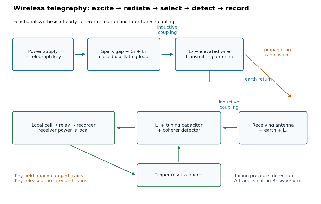
Functional transmit and receive chain for tuned spark wireless telegraphy
. Original functional synthesis of tuned spark wireless apparatus and early coherer reception. Arrows show functional transfer; local battery energy powers recording. Details.A filings coherer changes from high to low electrical resistance following electrical excitation. A local battery supplies the readout electric current; a tap resets the detector. It records events rather than the incident radio wave waveform.
Marconi described nickel and silver filings between silver plugs, with a cell and sensitive telegraph relay controlling a tapper and recorder.[ref]
Wireless Telegraphic Communication by Guglielmo Marconi. 1909 lecture, printed p. 197, Fig. 1 and following paragraph: coherer construction and local readout
A telegraph relay uses a small control electric current to switch a separate local electrical circuit. The recording mechanism's energy can therefore come from its own battery, rather than from the weak received signal. A sensitive trigger and a powerful readout serve different functions.
Guglielmo Marconi's 1909 lecture describes antennas with earth connections and separate coupled receiving circuits. His 1900 system coupled a closed capacitor–inductor–spark gap loop to a transmitting antenna. Coil spacing adjusted coupling; inductance and capacitance adjusted tuning. All four circuits were tuned together. By 1909 his company's stations mainly used magnetic receivers, rather than coherers.[ref]
Wireless Telegraphic Communication by Guglielmo Marconi. 1909 lecture, Figs. 2–3, 6 and 8 and associated paragraphs; receiver paragraph at Fig. 25
Those are a participant's retrospective descriptions, not a complete account of priority. An earth connection is part of this antenna arrangement; it is not a universal requirement for radio communication. Nor does tuning an isolated LC circuit ensure that its frequency remains unchanged when strongly coupled to another circuit. The coupled resonant circuit model quantifies that distinction.
In his 1909 lecture, Karl Ferdinand Braun recalled two experimental stations on Strasbourg forts in summer 1902. Known capacitances and calculated inductances set the transmitter tuning; the receiver searched for its two coupled oscillations. Its receiving coil fed a second coil in a tuned indicator circuit. Separating these coils increased both the sharpness of resonance and excitation intensity, until further separation reduced the response. The varied coil spacing was the control; transmitter coupling need not be loose for this receiver effect. For intensity measurements, Braun described an air-thermometer readout in the related resonant measuring apparatus.[ref]
Electrical Oscillations and Wireless Telegraphy by Karl Ferdinand Braun. 1909 lecture, printed p. 234: Strasbourg stations, coil-spacing test and air-thermometer readout
The comparison tests receiver coupling, not an unrestricted law that looser coupling always helps. The paragraph does not identify the particular indicator used in the coil-spacing test or give a response curve from which to reconstruct its optimum. The plotted curves below are an original linear model with stated losses, rather than invented historical measurements.
A spark gap can rapidly discharge a charged capacitor through an inductor. After excitation, the stored energy runs down through Joule heating, radiation and other losses. A key held down can permit repeated discharges: each discharge starts a damped train of rapid oscillations. The spark repetition frequency, the electrical oscillation frequency within each train, and the rate of keyed symbols are different quantities. Repetition does not make each train a maintained sinusoid.
An original lumped model replaces the conducting spark gap and other losses by a constant total electrical resistance in an isolated series RLC circuit. For electric charge on the capacitor, the Kirchhoff cycle law givesFor , its characteristic roots are , with , proving the stated damped form. The electric current has the same exponential decay scale. Its wave envelope falls by per cycle; the energy envelope falls twice as fast in the exponent. A maintained sinusoid instead requires continuing input power balancing losses.
With , and , the model gives , Q factor , amplitude time constant , and damped frequency . These are chosen component values. A real spark gap switches nonlinearly, an antenna radiates, and coupling exchanges energy between circuits; one constant- free decay does not model the complete transmitter. Rapid damping also broadens the frequency spectrum, which helps explain why short trains make sharp receiver selection difficult.
MIT's demonstration places two 120-turn coils face to face, each with a capacitor. A swept sinusoid drives one circuit; an oscilloscope observes the other circuit's capacitor electric potential difference. The sheet specifies and or , giving nominal resonant frequencies near and . It presents a procedure, not a measured dataset.[ref]
Mutual Inductance with Two Coils Resonant by Massachusetts Institute of Technology Technical Services Group. L5, “Mutual Inductance W/Two Coils Resonant”: apparatus, frequency sweep, secondary capacitor readout and nominal component values
A reproducible extension can test the same selection principle with the identical components of the coupled resonant circuit model. Prepare two separate series loops, measure their actual inductances, capacitances and coil electrical resistances, and include generator Thévenin resistance in the driven loop's total . Choose added resistors to make if the measured losses permit it. Include a known sense resistor within . Drive the first loop with a small function generator sinusoid; read the second loop's electric current as using an oscilloscope across the sense resistor. Here denotes the sense reading, distinct from the source electric potential difference in the model.
Sweep – slowly enough for transients to settle; record source frequency, source amplitude at the circuit terminals, and sense amplitude. Repeat at fixed coil spacing after changing one capacitor, then at fixed components after changing spacing. Turn the drive off to establish the background; rotate the receiving coil toward a right angle to test inductive coupling; restore its orientation and repeat to check drift. These are proposed controls, not observations reported by MIT. Keep probe loading small and account for it if not negligible. A grounded oscilloscope can electrically join the loops if attached to both: use an appropriately isolated differential input for any simultaneous primary measurement, or measure the primary separately.
Recovering deliberately chosen long and short generator bursts on the receiver trace demonstrates symbol timing. The essential inference is narrower than a long-distance radio test: nearby coils primarily exchange energy through mutual inductance in the near and far field regime dominated by the near field. Coil spacing, detuning and background controls distinguish this coupling from a direct wire connection or incidental pickup. They do not by themselves demonstrate reception of propagating radio waves in the radiation zone.
Let two series loops have inductances , capacitances , total electrical resistances , and reciprocal mutual inductance with . For a steady sinusoid of angular frequency , choose complex peak amplitudes with time convention . An ideal source of peak electric potential difference drives loop 1; loop 2 has no independent source. ThenEliminating proves the response formula. Reversing one coil changes the sign of and the relative wave phase, but leaves this amplitude response unchanged. The measured sense ratio is , with included in , not added a second time.
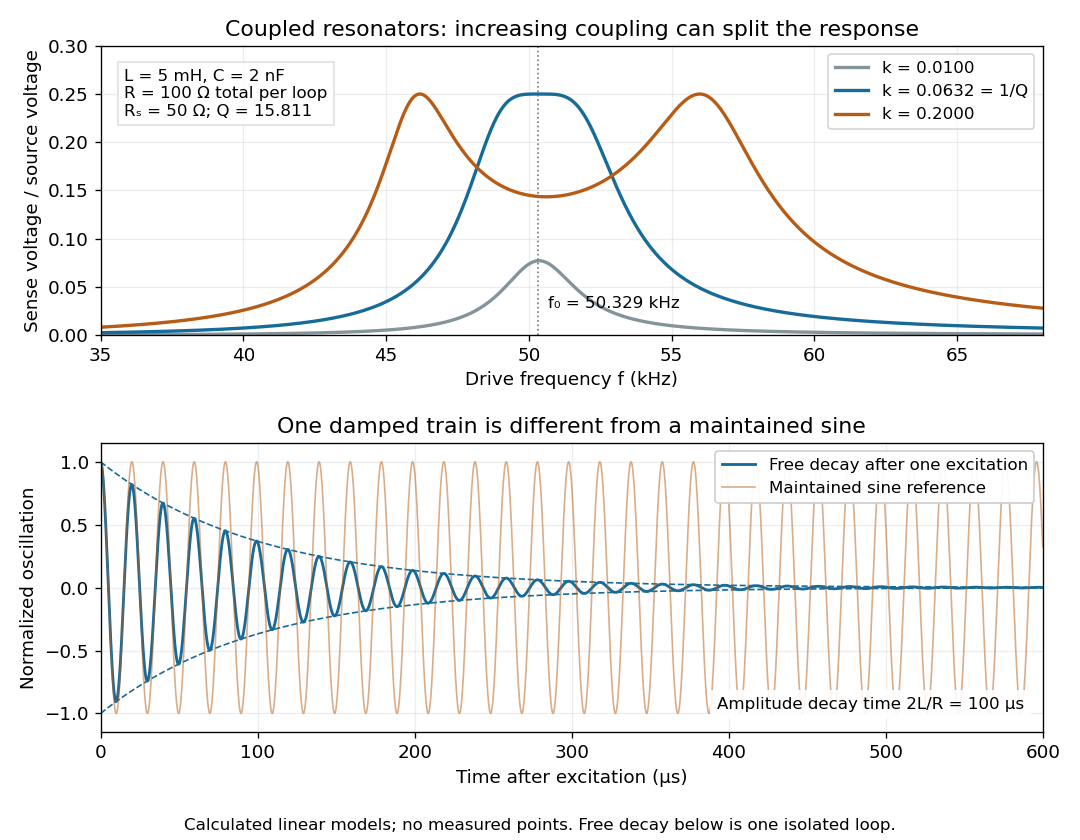
For identical loops at their uncoupled resonant frequency ,Writing makes this . Its derivative has the sign of , so response at this fixed frequency is largest when , equivalently . Too little coupling transfers little excitation; excessive coupling reduces the response at the original centre frequency. This is a fixed-frequency optimum, not a universal optimum over every possible receiver and drive frequency.
For the chosen values, gives . At source peak , the secondary peak electric current is and the sense peak electric potential difference is . The primary peak electric current is also , so source mean power is : each loop dissipates , checking conservation of energy. Here is the equivalent ideal source behind ; a generator's terminal reading must be converted using its measured Thévenin resistance.
In the lossless identical-loop limit, the normal modes have equal or opposite electric currents, making their effective inductances or . ThusAt these are and . Finite electrical resistance broadens and shifts the driven peaks, so the exact response formula, rather than these lossless values, generates the plot. Changing a capacitor moves the uncoupled tuning through : increasing it by lowers by the factor . The model explains why tuning and coupling must be adjusted together; it supplies no transatlantic propagation or detector-threshold prediction.
Articles by others on the same topic



A very cool thing about telecommunication is, besides how incredibly fast it advanced (in this sense it is no cooler than integrated circuit development), how much physics and information theory is involved in it. Applications of telecommunication implementation spill over to other fields, e.g. some proposed quantum computing approaches are remarkably related to telecommunication technology, e.g. microwaves and silicon photonics.
This understanding made Ciro Santilli wish he had opted for telecommunication engineering when he was back in school in Brazil. For some incomprehensible reason, telecommunications was the least competitive specialization in the electric engineering department at the time, behind even power electronics. This goes to show both how completely unrelated to reality university is, and how completely outdated Brazil is/was. Sad stuff.