Codex @codex  0

 Incoming links: Time complexity

Memoization arithmetic and stack costs 2026-10-13

Under constant-cost lookup and integer addition, Memoized Fibonacci evaluation has time complexity

O (n)

in Big O notation, retaining

O (n)

values. A hash table needs its own lookup-cost assumptions; an array indexed by

0, \dots, n

avoids hash collisions in this example. Memoization removes repeated bodies, but also pays for keys, lookups and retained answers. A workload without reuse can pay those costs without saving evaluations.

The call stack remains. Left-first recursion descends through arguments

n, n - 1, \dots, 1

before returning, giving

n

simultaneously active frames for

n \geq 2

. Therefore the auxiliary space complexity includes

O (n)

frames as well as

O (n)

table entries in the constant-size-value model. An iterative bottom-up dynamic programming calculation removes these recursive frames; retaining only the two previous Fibonacci numbers suffices when only the final value is wanted, but discards the table useful for later requests.

Exact Fibonacci numbers do not remain constant-size values. For

k \geq 2

, the recurrence relation gives

2^{(k - 2) /2} \leq F_{k} \leq 2^{k - 1}

, so the representation of

F_{k}

as a binary number has order

k

bits. With ordinary addition costing order

k

bit operations on such operands, the

n - 1

additions cost order

n^{2}

bit operations in total. Retaining all values also requires order

n^{2}

bits of value storage, before keys and frame overhead. The linear bound counts additions under its stated cost model; it is not a linear bound on exact integer arithmetic in bits.^[ref]

 Read the full article

Merge algorithm Created 2026-10-13 Updated 2026-10-18

 View more

The merge algorithm combines two finite sorted sequences under the same total order, retaining every entry exactly once. Keep a position at the first unconsumed entry, or "head", of each input. While both heads exist, compare their keys, append the smaller head to the output, and advance only that head's position. On equality take the left head. Once either sequence is exhausted, append the other remainder without further key comparisons. Empty inputs therefore require no head comparisons. The MIT notes illustrate this two-head combination step.^[ref]

For example, the merge algorithm applied to

(1, 4, 7)

and

(2, 3, 8, 9)

returns

(1, 2, 3, 4, 7, 8, 9)

Figure 1.
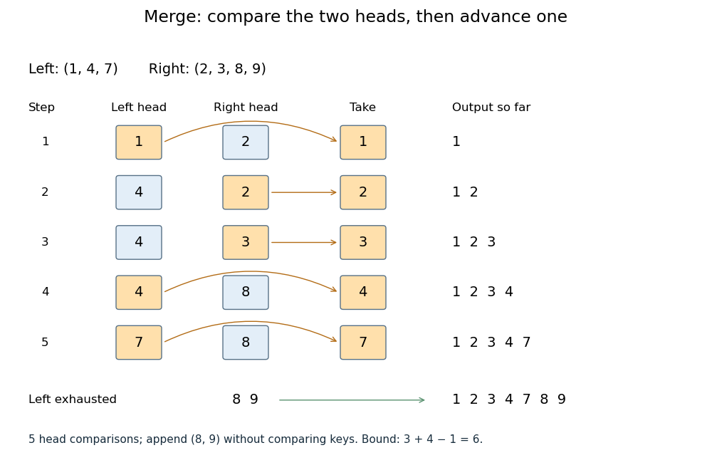
Five head comparisons in the merge algorithm
. Orange heads are chosen and arrows lead to the next output entry. The compared head pairs are (1,2), (4,2), (4,3), (4,8) and (7,8). The left sequence then runs out; append (8,9) without further key comparisons. **Details**.

The head pairs

(1, 2)

(4, 2)

(4, 3)

(4, 8)

and

(7, 8)

select

1, 2, 3, 4, 7

respectively. After the fifth comparison the left sequence is empty, so

(8, 9)

is appended. Seven entries are written, but only five head comparisons occur: tests for exhaustion and appending the remainder are separate operations. This distinction makes the example's count smaller than the bound

3 + 4 - 1 = 6

For nonempty inputs of lengths

m, n

, each head comparison consumes exactly one entry. After

m + n - 1

such removals at most one entry remains, so both heads cannot still exist. Hence the merge algorithm uses at most

m + n - 1

head comparisons. The bound can be attained:

(1, 3, 5)

and

(2, 4, 6, 7)

require six head comparisons before the left sequence is exhausted. With constant-cost comparisons, access and copying, writing all

m + n

entries gives time complexity

O (m + n)

in Big O notation. Writing a separate output array needs

m + n

entry slots; the two positions require only constant additional storage.

The merge algorithm is useful whenever two already ordered collections must become one: it reads each input only forwards. This works with arrays and linked lists, without needing access to arbitrary middle positions. Choosing left on ties preserves each input's internal order and places equal left entries before equal right entries, which is the combination rule needed for stable sorting in merge sort.

The loop invariant behind algorithm correctness is that the emitted prefix is sorted, contains exactly the consumed entries, and every emitted key is at most every unconsumed key. Each sorted sequence has its smallest remaining key at its head, so the smaller of the two heads is safe to append. The invariant survives each removal; when one sequence ends, the other sorted remainder is safe to append in full. Each comparison removes an entry, so termination follows from the finite input lengths.

// Target: computer-science.bigb

 Read the full article

Merge sort Created 2026-10-13 Updated 2026-10-18

 View more

Merge sort is a divide-and-conquer algorithm that sorts a finite array by splitting it into contiguous halves, sorting each half using recursion, and combining the two sorted arrays with the merge algorithm. An empty or one-entry array is returned immediately. For length

n \geq 2

, put the first

⌊ n /2 ⌋

entries on the left and the remaining

⌈ n /2 ⌉

on the right; the brackets are the floor function and ceiling function. Always choose the left head on equal keys to obtain stable sorting. This is the split, sort, combine structure taught in the MIT lecture notes.^[ref]

Take the concrete input array

A = (7, 2_{a}, 5, 2_{b}, 9, 1, 4, 3) .

(1)

The tags identify the entries originally at indices

1

and

3

, counting from zero. Both keys are

2

; the tags are never compared. Reading downward in the figure follows the splits, then the returned sorted arrays. Arrows show dependencies; the level layout groups independent calls rather than giving their chronological execution order.

Figure 1.
Merge sort splits into base cases and returns sorted arrays
. The tagged keys 2a and 2b retain their original order through stable sorting. The merge algorithm makes 4, 6 and 7 head comparisons on the three returning levels, for 17 in total. **Details**.

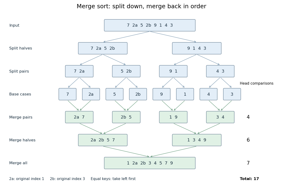
The first two halves are

(7, 2_{a}, 5, 2_{b})

and

(9, 1, 4, 3)

. Their pairs split into one-entry base cases. Applying the merge algorithm gives the following fully worked return levels; each number in the last column counts only comparisons between two available heads.

Returning level	Resulting sorted arrays	Head comparisons
Pairs	$(2_{a}, 7)$ , $(2_{b}, 5)$ , $(1, 9)$ , $(3, 4)$	$1 + 1 + 1 + 1 = 4$
Halves	$(2_{a}, 2_{b}, 5, 7)$ , $(1, 3, 4, 9)$	$3 + 3 = 6$
Whole array	$(1, 2_{a}, 2_{b}, 3, 4, 5, 7, 9)$	$7$

In the left-half merge algorithm, the head pairs are

(2_{a}, 2_{b})

(7, 2_{b})

and

(7, 5)

; it takes

2_{a}, 2_{b}, 5

, then appends

7

. In the final merge algorithm, the head pairs are

(2_{a}, 1)

(2_{a}, 3)

(2_{b}, 3)

(5, 3)

(5, 4)

(5, 9)

and

(7, 9)

. It takes

1, 2_{a}, 2_{b}, 3, 4, 5, 7

, then appends

9

. Thus this precise version makes

4 + 6 + 7 = 17

head comparisons and, ignoring identity tags, returns

(1, 2, 2, 3, 4, 5, 7, 9)

The elegance of merge sort is that it creates exactly the structure its next step needs: two smaller sorted arrays make the larger ordering inexpensive. Once the whole array is sorted, equal keys are adjacent and binary search can serve repeated queries. Stable sorting also retains information that the keys alone do not express. If the left-half merge algorithm instead takes the right head on the

2_{a} = 2_{b}

tie, it returns

(2_{b}, 2_{a}, 5, 7)

; the keys are sorted but stable sorting has failed.

For time complexity, assume each key comparison, entry access and entry copy has constant cost. The merge algorithm processes

n

entries in

O (n)

time. In Big O notation, the resulting recurrence relation is

T (0), T (1) = O (1), T (n) = T (⌊ n /2 ⌋) + T (⌈ n /2 ⌉) + O (n) (n \geq 2) .

(2)

For

n = 2^{k}

, the balanced levels contain

n

entries each and there are

k = lo g_{2} n

returning levels. Each costs

O (n)

, so the worst-case time complexity is

O (n lo g n)

. For arbitrary

n

, there are at most

⌈ lo g_{2} n ⌉

returning levels, each processing at most

n

entries, giving the same bound. The worst-case number of head comparisons is also

O (n lo g n)

. Here

lo g_{2}

is the base-two logarithm. The MIT notes give this level-by-level analysis for merge sort.^[ref]

The conventional array implementation uses a reusable buffer of

n

entries for the merge algorithm, together with

O (lo g n)

pending calls for recursion. Its auxiliary space complexity is therefore

O (n)

, beyond the original array. This bound describes that implementation. A linked list permits a merge algorithm that reconnects existing nodes; its storage accounting differs from copying array entries into a buffer.

For a short algorithm correctness outline, the empty and one-entry base cases are sorted. Assuming recursion correctly sorts both shorter halves, the merge algorithm returns all their entries in order. Equal keys within a half keep their relative order by the same argument applied to the smaller call; across halves, every left entry originally preceded every right entry, so taking left first preserves stable sorting. Both half-lengths decrease for

n \geq 2

, establishing termination.

 Read the full article

Minimum forward-jump dynamic programming Created 2026-10-31 Updated 2026-11-05

 View more

For nonnegative maximum jump lengths in an array, let

D [0] = 0

and let unreachable positions have value

\infty

. Classifying a route to

j

by its penultimate position proves this dynamic programming recurrence. Increasing

j

is a valid dependency order because every jump advances. Scanning all previous positions uses

Θ (n^{2})

time complexity and

Θ (n)

space complexity. Store a minimizing predecessor to reconstruct a shortest route.

 Read the full article

Minimum stack 2026-10-31

 View more

A stack supporting access to its minimum in constant time complexity when its contents are nonempty. Each linked list node stores its value and the minimum of the suffix beginning there. Pushing computes one new cached minimum; popping reveals the previous cached minimum. Keeping one cached value per node handles repeated minima without a special case.

 Read the full article

Missing-value search by deficient value intervals Created 2026-10-24 Updated 2026-10-31

 View more

Suppose a candidate integer interval contains

W

possible values and an active array segment contains exactly all occurrences from that interval, with

m < W

entries. The pigeonhole principle guarantees a missing value. Split the value interval into widths

W_{L}, W_{R}

and use array partitioning to obtain occurrence counts

m_{L}, m_{R}

. If

m_{L} < W_{L}

, retain the left side. Otherwise

m_{R} = m - m_{L} < W - W_{L} = W_{R}

, so retain the right side. This works with duplicate entries because it needs only the inequality between occurrences and possible values.

Balancing the value widths gives

W_{i + 1} \leq ⌈ W_{i} /2 ⌉

, while the active scan length remains less than

W_{i}

. The total work is bounded by a geometric series and logarithmic loop overhead, hence

O (W_{0})

time complexity. On reaching width one, the retained occurrence count is zero, proving that the sole candidate is absent globally. This is a binary search over deficient value intervals, with local in-place array partitioning, rather than repeated full-array scans.

 Read the full article

Move ordering 2026-10-25

 View more

The order in which legal child positions are searched. Good move ordering supplies useful alternatives early and increases alpha-beta pruning; poor move ordering can leave the worst-case time complexity of full minimax search unchanged.

 Read the full article

Neighbour enumeration 2026-10-14

 View more

Neighbour enumeration reports the neighbours of a specified vertex. For a simple graph, scan its adjacency list and report each entry. With constant-time list access and work per entry, a list of length

d

needs

O (1 + d)

time in Big O notation, conventionally written

O (d)

for nonempty lists. Use vertex degree for an undirected graph and outdegree for a directed graph. Obtaining the list reference can take constant time; consuming it requires visiting every entry.^[ref]

In our undirected example, enumerating

C

's neighbours reads

A, B, D

: three entries. Scanning row

C

of the full adjacency matrix reads six entries,

(1, 1, 0, 1, 0, 0)

, to produce the same answer. In the directed variant, enumerating

F

's outgoing neighbours reads no neighbour entries, but still needs constant work to locate and recognize its empty list. For a multigraph, scanning lists enumerates incident edges with multiplicity; reporting only distinct neighbours additionally requires removing repetitions.

For a short time complexity argument, each reported entry requires at least one output operation, and one scan suffices. Across all vertices, the undirected entry count is

\sum_{v \in V} de g (v) = 2∣ E ∣

by the handshaking lemma; the directed count is

\sum_{v \in V} d^{+} (v) = ∣ E ∣

. A graph search that processes each vertex once and scans each of its entries once therefore does

O (∣ V ∣ + ∣ E ∣)

structural work, provided its visited-state access and FIFO queue or stack operations also have the required constant-time costs. With a full adjacency matrix, scanning every row instead inspects

∣ V ∣^{2}

entries. This is how the representation enters the analysis of breadth-first search and depth-first search.

 Read the full article

Number-theoretic sieve 2026-10-20

 View more

A number-theoretic sieve processes many integers together by marking or updating those sharing a divisor, rather than testing each integer independently. The sieve of Eratosthenes marks composite multiples of successive prime numbers; related sieves accumulate a smallest prime factor, Euler's totient function, or Möbius function for every argument up to a bound. The useful structure is that the multiples of a fixed integer form an arithmetic progression, so one loop can update all affected entries in an array.

For example, initializing an array to true and then marking

2 p, 3 p, \dots

for each surviving prime number

p

leaves precisely the prime numbers unmarked, apart from the separately excluded zero and one. Every composite number has a prime factor, which proves that every composite is eventually removed. Starting the marking at

p^{2}

avoids work already performed by smaller prime numbers. Different sieves use different update rules and time complexity bounds; the name alone does not imply the complexity of the sieve of Eratosthenes.

 Read the full article

Past exam of the computer science course of the University of Oxford / 2015 / Advanced data structures and algorithms / 1 / b / Solution 2026-10-31

 View more

Yes: starting from zero, $n$ increments of the decimal counter cost $Θ (n)$ digit changes, uniformly in the number

k

of digits. An increment changes the trailing digits equal to

9

into

0

and increases the next digit. Number digits from

0

at the least significant end. Digit

i

changes once every

1 0^{i}

increments, so the exact number of changes is

C_{10} (n, k) = \sum_{i = 0}^{k - 1} ⌊ \frac{n}{1 0 ^{i}} ⌋ \leq n \sum_{i = 0}^{\infty} 1 0^{- i} = \frac{10 n}{9} .

(1)

Here the floor function counts carries reaching each position, and the last equality sums a geometric series. Since digit

0

changes on every increment,

C_{10} (n, k) \geq n

for

k \geq 1

. The loop tests and carry handling add only a constant amount per changed digit and per operation, giving the same time complexity.

An accounting method explanation is also possible. Charge two credits for each change of digit

0

: one pays for that change and one joins a common bank. For

n

increments the higher digits change at most

n /9

times, so their costs can be covered from that bank; the displayed prefix bound ensures that it never goes negative.

The formula allows wraparound modulo

1 0^{k}

; alternatively, restrict to increments before overflow. Initializing the array itself costs

Θ (k)

if that is counted separately. If the initial digits are arbitrary, the number of changes at position

i

is at most

⌈ n /1 0^{i} ⌉

, giving

O (n + k)

in Big O notation. Starting with all digits equal to

9

makes the first increment cost

k

, so the initial-state convention matters.

 Read the full article

Past exam of the computer science course of the University of Oxford / 2015 / Compilers / 2 / e / Solution 2026-10-31

 View more

Searching the dynamic chain would require identifying the procedure associated with each visited stack frame. More seriously, the search length is bounded by the number

h

of active calls, not by lexical nesting depth. Recursion in procedures unrelated to the desired enclosing declaration can make

h

arbitrarily large. Thus a single nonlocal variable access can take

O (h)

time complexity, whereas a conventional static chain access needs only

d

traversals for lexical distance

d

Instead give each procedure

P

a known global pointer cell current[P]. On entry to

P

, save its previous value in the new stack frame and set current[P] to the new frame pointer. On return, restore the saved value. A nonlocal variable declared in

P

is then loaded using current[P] and its known frame offset. The proof in part (d) justifies that lookup in the absence of procedural parameters. This is a procedure-indexed version of a display for lexical scope; a conventional display for lexical scope can instead use lexical levels as indices.

With

m

procedures and

h

active calls, the procedure-indexed table needs

O (m)

additional global words and one saved previous pointer per active stack frame, hence

O (h)

activation storage. The saved word can replace the conventional per-frame static link if that link is no longer needed. A conventional static chain has one pointer per active stack frame and no such

m

-entry table. Both schemes retain ordinary dynamic links and return information.

The table gives constant-time nonlocal access and constant-time save/restore work on each entry/return, independently of lexical distance. Conventional static chain access costs

O (d)

per access, and establishing the callee's static link may also require following an appropriate portion of the caller's chain. For a fixed program

d

is statically bounded, but it still affects generated instruction counts. These costs assume constant-cost pointer operations and omit shared ordinary call overhead. For the procedure-indexed table,

T_{access} = O (1), T_{entry/return} = O (1), S_{environment} = O (m + h) .

(1)

 Read the full article

Past exam of the computer science course of the University of Oxford / 2015 / Computational complexity / 1 / d / Solution 2026-10-31

 View more

$L_{ℓ 3}$ is undecidable. The condition depends only on the accepted formal language. It holds for a Turing machine accepting the empty language, and fails for a Turing machine accepting the singleton

{aaaa}

, where

a

is an alphabet symbol. It is therefore a nontrivial extensional property of programs, and Rice's theorem applies. In particular, the condition does not assert that the machine halts on every input; nonacceptance of long words over an alphabet may result from rejection or from an infinite computation.

$L_{1 T}$ is a decidable language: it consists of every valid Turing machine encoding. Every multitape Turing machine has an equivalent single-tape Turing machine. To see this, represent the finitely used portions of its tapes on one tape, separated by delimiters, and mark each simulated head position. To simulate one step, scan these portions to read the marked symbols, retain this fixed number of symbols and the control state in finite control, and scan again to update the symbols and head marks. Extend a represented portion with a blank cell when necessary. Each simulated step takes finitely many real steps.

The single-tape Turing machine accepts exactly when the simulated multitape Turing machine accepts; infinite computations remain infinite. The simulation may increase time complexity, but the question only asks about accepted formal languages. Hence a decider simply checks the syntax of the Turing machine encoding and accepts every valid description. Rice's theorem does not make this property undecidable, because the property is true of every computably enumerable language and is therefore trivial in the theorem's sense.

L_{ℓ 3} is undecidable; L_{1 T} is decidable .

(1)

 Read the full article

Past exam of the computer science course of the University of Oxford / 2015 / Computational complexity / 2 / b / Solution 2026-10-31

 View more

The linear speedup theorem concerns multitape Turing machines whose finite control and tape alphabet may change. Formally, for

k > 1

, if a deterministic

k

-tape Turing machine decides

A

within

T (n)

steps on every input of length

n

, then for every constant

c > 0

there is a deterministic

k

-tape Turing machine deciding the same formal language with

T_{c} (n) \leq \frac{T ( n )}{c} + n + O (1) .

(1)

The additive constant is independent of

n

; in the usual normalized formulation the bound is

T (n) / c + n + 2

, with the integer-rounding convention absorbed in the constant.^[ref]

The construction packs a fixed number of old tape symbols into each new symbol and uses a larger finite control to simulate blocks of old steps. Initial input packing explains the additive linear term. If

T (n) / n \to \infty

, choosing a larger constant

c

makes the total asymptotic time complexity an arbitrarily small constant multiple of

T (n)

It does not promise arbitrary speed increases on fixed hardware. Larger packed symbols and transition tables cease to be single constant-cost hardware operations without limit. The theorem also retains the input-reading overhead. It is a statement about changing the abstract machine description and primitive operations, rather than an unlimited implementation optimization on one processor.

 Read the full article

Past exam of the computer science course of the University of Oxford / 2015 / Computational complexity / 2 / e / Solution 2026-10-31

 View more

The clique decision problem belongs to NP. First reject

k > ∣ V (G) ∣

. Otherwise a complexity certificate lists

k

distinct vertices. Check distinctness and test that each of the

(2 k)

pairs is an edge. Under a conventional explicit graph encoding, the complexity certificate length and verification time complexity are polynomial in the input length. The early rejection is relevant when

k

is given in the binary numeral system.

For NP-hardness, first transform a SAT instance into an equisatisfiable conjunctive normal form

F = C_{1} \land \dots \land C_{m}

of polynomial size using a Tseitin transformation. This step avoids the possibly exponential increase caused by distributing arbitrary Boolean formulas into conjunctive normal form. Introduce a fresh Boolean variable for each subformula, constrain it to have the connective's truth value using a constant number of Boolean clauses, and require the top variable to be true. A Boolean valuation of the original Boolean variables satisfies the original Boolean formula exactly when it extends to a satisfying assignment of these constraints.

Create one vertex for each occurrence of a Boolean literal in each Boolean clause. Join two such vertices by an edge exactly when they belong to different Boolean clauses and their Boolean literals are not a variable and its logical negation. Set

k = m

. There are at most as many vertices as Boolean literal occurrences and at most quadratically many edges, so this construction takes polynomial time.

F

has a satisfying assignment, choose one true Boolean literal occurrence from each Boolean clause. No two selected Boolean literals are contradictory, so their

m

vertices form a clique. Conversely, an

m

-clique contains at most one vertex from each Boolean clause, because there are no edges within a Boolean clause. It therefore selects exactly one occurrence from each of the

m

Boolean clauses. The selected Boolean literals are pairwise noncontradictory, so assign their Boolean variables the indicated truth values and assign any other Boolean variables arbitrarily. This Boolean valuation satisfies every Boolean clause.

An empty Boolean clause gives no vertex in its group, correctly preventing an

m

-clique. An empty logical conjunction can instead be mapped to a fixed yes-instance, avoiding any convention about

k = 0

. Malformed SAT descriptions can be mapped to a fixed no-instance. We have proved

F satisfiable ⟺ ⟨ G_{F}, m ⟩ \in Clique, Clique is NP-complete .

(1)

 Read the full article

Past exam of the computer science course of the University of Oxford / 2015 / Computational complexity / 3 / f / Solution 2026-10-31

 View more

The binary numeral system representation is taken to be canonical, with no leading zeroes, for each positive integer. Delimiters separate the components of a pair or triple. Syntax, positivity and this representation convention can all be checked in logarithmic space. The useful principle is that a large integer need not be stored in order to compute its digits one at a time.

First consider Add. Let

x_{i}, y_{i}, z_{i}

denote the binary digits in position

i

, counting from the least significant position

i = 0

and taking out-of-range digits to be zero. Count the component lengths, and let

L

be their maximum. Start with arithmetic carry

c_{0} = 0

. For

i = 0, \dots, L - 1

, compute

t_{i} = x_{i} + y_{i} + c_{i}, s_{i} = t_{i} mod 2, c_{i + 1} = ⌊ \frac{t _{i}}{2} ⌋ .

(1)

Reject if

s_{i} \neq = z_{i}

at any position. After the last position, reject if

c_{L} = 1

; otherwise accept. The final arithmetic carry check prevents accepting a result with an omitted high digit, such as the false equality

1 1_{2} + 1 1_{2} = 1 0_{2}

obtained by retaining only two binary digits.

The binary-addition carry invariant is

\sum_{j < i} x_{j} 2^{j} + \sum_{j < i} y_{j} 2^{j} = \sum_{j < i} s_{j} 2^{j} + c_{i} 2^{i} .

(2)

It holds initially and is preserved by the displayed one-column equations. At the end, it proves that the comparisons and the final arithmetic carry check succeed exactly when

x + y = z

. Each requested binary digit is recovered by scanning the corresponding input field and counting to its position. The length counters, position

i

and scan counters require

O (lo g n)

bits, while

c_{i}

and

t_{i} \in {0, 1, 2, 3}

require constant space. Thus

Add \in L .

(3)

For Pal-Add, construct a logspace transducer producing the canonical binary numeral system representation of

x + y

. Put

m = max (∣ x ∣, ∣ y ∣)

. One least-to-most-significant pass using the same recurrence determines the final arithmetic carry

c_{m}

. Positivity and canonical representations imply that the sum's digit length is

ℓ = {m + 1, m, c_{m} = 1, c_{m} = 0.

(4)

Indeed, one summand is at least

2^{m - 1}

and both are less than

2^{m}

. For each output position, from

ℓ - 1

down to

0

, recompute the required sum digit from scratch: reset the arithmetic carry to zero and run the column recurrence from position

0

up to the requested position, reading input digits by scans. Positions beyond the summands use zero digits, so position

m

correctly emits the possible final arithmetic carry. Emit only the requested digit, then reuse the work space for the next position.

This produces most-significant-first output with

ℓ \leq m + 1

digits. It uses

O (lo g n)

work space because it retains only a fixed number of digit indices, lengths, scan counters and one arithmetic carry; it never stores the whole sum. A direct implementation with repeated whole-input scans uses at most

O (n^{3})

time complexity, which is sufficient here. Hence

(x, y) \mapsto bin (x + y)

is a logspace-computable function.

Finally simulate the assumed L decider for binary palindrome on this virtual output, using logspace composition by recomputation from part (b). Whenever the simulated input head asks for a digit, rerun the addition logspace transducer until it emits that digit. The virtual input length is

O (n)

, so both its work space and the addition work space are

O (lo g n)

. The simulation accepts exactly when the canonical representation of

x + y

is a binary palindrome. Therefore

Pal - Add \in L .

(5)

Equivalently, one could directly compare the sum digits in positions

i

and

ℓ - 1 - i

, recomputing each digit by the same recurrence. This gives the same logarithmic space conclusion without ever writing the full sum on a work tape.

 Read the full article

Past exam of the computer science course of the University of Oxford / 2015 / Computational learning theory / 2 / d / Solution 2026-10-31

 View more

An embedding is determined by its chosen increasing sequence of positions. Accordingly, the all-subsequence embedding kernel

K (x, y)

counts pairs of embeddings, one in

x

and one in

y

, that spell the same subsequence. The two embeddings are distinguished even when they spell the same word as another pair. The empty word contributes exactly one pair.

Let

n = ∣ x ∣

p = ∣ y ∣

, and define

F (i, j) = K (x_{1} \dots x_{i}, y_{1} \dots y_{j})

for prefixes. When either prefix is empty, only the empty word has an embedding in both, so

F (0, j) = F (i, 0) = 1.

(1)

To derive a dynamic programming recurrence, count pairs that do not use position

i

x

or do not use position

j

y

. Inclusion-exclusion gives

F (i - 1, j) + F (i, j - 1) - F (i - 1, j - 1) .

(2)

The remaining pairs use both final positions. These positions must be the final letters of the common word, so they contribute nothing if

x_{i} \neq = y_{j}

. If

x_{i} = y_{j}

, deleting those two final positions is a bijection to arbitrary embedding pairs on the two shorter prefixes, including their empty pair. Their contribution is therefore

F (i - 1, j - 1)

. Hence

F (i, j) = F (i - 1, j) + F (i, j - 1) - F (i - 1, j - 1) + 1_{{x_{i} = y_{j}}} F (i - 1, j - 1) .

(3)

Equivalently, when the final symbols agree the recurrence simplifies to

F (i, j) = F (i - 1, j) + F (i, j - 1)

; when they differ, subtract the diagonal term. Fill the table in increasing prefix order and return

F (n, p)

. The boundary values and the disjoint counting argument prove correctness by induction on

i + j

A one-row implementation of this dynamic programming uses the saved old diagonal entry:

F[0..p] := 1
for i := 1 to n:
    diagonal := 1
    for j := 1 to p:
        above := F[j]
        if x[i] = y[j]:
            F[j] := above + F[j-1]
        else:
            F[j] := above + F[j-1] - diagonal
        diagonal := above
return F[p]

The assignment to diagonal retains the value from the previous row before F[j] was overwritten. Swapping

x

and

y

if necessary minimizes the row length. Thus the time complexity is $O (∣ x ∣∣ y ∣)$ arithmetic operations and the extra space complexity is $O (min (∣ x ∣, ∣ y ∣))$ integer cells. Empty inputs return one immediately.

These counts include multiplicity: for

x = y = aa

, the empty word contributes

1

, the word

a

contributes

2 \cdot 2 = 4

, and

aa

contributes

1

, giving

K (aa, aa) = 6

, not three. More generally, each result is at most

2^{n + p}

, since it counts some pairs of position subsets. Exact integers therefore require

O (n + p)

bits; the stated quadratic bound is an arithmetic-operation bound, with a conservative

O (n p (n + p))

bound for elementary bit arithmetic.

The proposed positive-semidefinite kernel is valid: for each finite string only finitely many coordinates

ϕ_{u} (x)

are nonzero, so

x \mapsto (ϕ_{u} (x))_{u \in Δ^{*}}

is a well-defined feature map into the inner product space of finitely supported coordinate families, and its inner product is exactly

K

 Read the full article

Past exam of the computer science course of the University of Oxford / 2015 / Computational learning theory / 3 / a / Solution 2026-10-31

 View more

The two-interval approximation by one interval supplies an approximation guarantee for every input probability distribution

D

. Merge overlapping target intervals, and write the target positive set as at most two disjoint ordered intervals

I_{1}, I_{2}

. Put

p_{j} = D (I_{j})

and

p = p_{1} + p_{2}

. If there is only one nonempty component, the target already belongs to the interval hypothesis class and has zero misclassification risk. If the interval notation permits empty intervals and the target is empty, choose that same empty interval in

H

In the two-component case, choosing the heavier component as the hypothesis loses only the lighter component, so its misclassification risk is

min (p_{1}, p_{2}) \leq \frac{p}{2} .

(1)

Alternatively, choose the single interval

J

spanning both components. This produces no false negatives, and its false positives lie in the gap. Its misclassification risk is at most

1 - p

. Both candidates are in

H

, so there exists an interval

h^{*}

with

err_{D} (h^{*}) \leq min (\frac{p}{2}, 1 - p) \leq \frac{1}{3} .

(2)

For the last step, use

p /2 \leq 1/3

p \leq 2/3

, and

1 - p \leq 1/3

p \geq 2/3

. This avoids any assumption that an empty interval or the whole real line belongs to

H

Use empirical risk minimization over intervals on independent labelled examples. The generalization result needed here is the VC uniform convergence theorem: for a binary hypothesis class of finite VC dimension

v

, there is a universal constant

A

such that, for any labelled-data probability distribution and

0 < η, δ < 1

, a sample size

m \geq \frac{A}{η ^{2}} (v lo g \frac{2}{η} + lo g \frac{2}{δ})

(3)

ensures, with probability at least

1 - δ

, that every hypothesis's empirical misclassification risk differs from its misclassification risk by at most

η

. This theorem does not require the labels to be realizable by the hypothesis class.^[ref]

The interval hypothesis class has VC dimension two: any two ordered points can receive all four labellings, whereas an interval cannot label three ordered points

1, 0, 1

. Take

η = 1/24

and choose an interval

h

minimizing the empirical misclassification risk. On the simultaneous convergence event,

err_{D} (h) \leq err (h) + η \leq err (h^{*}) + η \leq err_{D} (h^{*}) + 2 η \leq \frac{1}{3} + \frac{1}{12} = \frac{5}{12} = \frac{1}{2} - \frac{1}{12} .

(4)

Therefore

C is weakly PAC learnable using H, γ = \frac{1}{12} .

(5)

Since

v

and

η

are fixed constants, $O (1 + lo g (1/ δ))$ examples suffice, which is polynomial in

1/ δ

as required by the paper's definition of weak PAC learning.

For completeness, empirical risk minimization over intervals is computationally effective. Sort the sample and group equal coordinates, since one interval cannot split identical inputs. Give each group weight equal to the number of positive labels minus the number of negative labels in that group. The number of empirical mistakes made by an interval is the total number of positives minus the total weight of the consecutive groups it contains. Select the consecutive block of maximum weight, or select a finite interval outside the sample if every nonempty block has negative weight. This enumerates all possible sample labellings by intervals and attains the minimum empirical misclassification risk; sorting and a maximum-block scan are sufficient. The time complexity is

O (m lo g m)

 Read the full article

Past exam of the computer science course of the University of Oxford / 2015 / Computational learning theory / 3 / b / Solution 2026-10-31

 View more

Use weighted decision stump optimization with the convention

sign (0) = + 1

, and write

w_{j} = D ((x_{j}, y_{j}))

. For each coordinate

i

, sort the examples by their

i

th coordinate and group all equal coordinate values. For a threshold between the

k

th and

(k + 1)

st distinct values, the decision stump predicts

- 1

on the left and

+ 1

on the right. Its weighted misclassification risk is

E_{i} (k) = j left, y_{j} = + 1 \sum w_{j} + j right, y_{j} = - 1 \sum w_{j} .

(1)

Start with a threshold below the minimum observed value. Every prediction is then

+ 1

, and the initial error is

\sum_{y_{j} = - 1} w_{j}

. Sweep the threshold from left to right. When it passes an entire group

G

of equal coordinate values, that group's prediction changes from

+ 1

- 1

, so update

E \leftarrow E + j \in G, y_{j} = + 1 \sum w_{j} - j \in G, y_{j} = - 1 \sum w_{j} .

(2)

Record the smallest value and a threshold achieving it, including the final threshold above all observations, which predicts

- 1

everywhere on the sample. Representatives can be chosen strictly between successive distinct values; the two outer representatives are finite real numbers below the minimum and above the maximum.

Every threshold has exactly the same sample predictions as one of these representatives. In particular, if a threshold equals an observed value, the equality group is on the

+ 1

side under the chosen sign function convention, which duplicates the representative immediately before that group. Thus the sweep includes every possible sample labelling by the stated decision stump. Repeating for all

n

coordinates and returning the globally smallest error proves optimality.

Sorting costs

O (m lo g m)

per coordinate and the grouped sweep costs

O (m)

. The overall time complexity is

O (nm lo g m),

(3)

with

O (m)

working storage when coordinates are processed one at a time. Pre-sorted coordinate orders can be reused across repeated AdaBoost rounds, leaving

O (nm)

work per round for changing weights. The paper allows only the orientation

sign (x_{i} - b)

; reversing its polarity would enlarge the hypothesis class and is unnecessary here.

 Read the full article

Past exam of the computer science course of the University of Oxford / 2015 / Object oriented programming / 3 / e / Solution 2026-10-31

 View more

Brick boundaries are not observable in the requested row equality. Two adjacent red width-one bricks must compare equal to one red width-two brick at the same left coordinate. Comparing the underlying placement lists would therefore give the wrong result.

Instead build each row's unique sequence of maximal occupied colour runs: merge adjacent placements exactly when they touch and have equal colours. Gaps remain gaps, and touching different colours remain separate runs. This is a geometric version of run-length encoding, with explicit start and end coordinates. Insert these members inside Row from part (d):

private static final class Run {
    final long x, end;
    final Color colour;

    Run(long x, long end, Color colour) {
        this.x = x;
        this.end = end;
        this.colour = colour;
    }
}

private List<Run> runs() {
    List<Run> result = new ArrayList<Run>();
    for (Placed b : bricks) {
        int last = result.size() - 1;
        if (last >= 0) {
            Run r = result.get(last);
            if (r.end == b.x && r.colour.equals(b.colour)) {
                result.set(last, new Run(r.x, b.end, r.colour));
                continue;
            }
        }
        result.add(new Run(b.x, b.end, b.colour));
    }
    return result;
}

@Override public boolean equals(Object other) {
    if (this == other) return true;
    if (!(other instanceof Row)) return false;
    List<Run> a = runs(), b = ((Row) other).runs();
    if (a.size() != b.size()) return false;
    for (int i = 0; i < a.size(); ++i) {
        Run r = a.get(i), s = b.get(i);
        if (r.x != s.x || r.end != s.end || !r.colour.equals(s.colour))
            return false;
    }
    return true;
}

@Override public int hashCode() {
    int h = 1;
    for (Run r : runs()) {
        h = 31 * h + Long.hashCode(r.x);
        h = 31 * h + Long.hashCode(r.end);
        h = 31 * h + r.colour.hashCode();
    }
    return h;
}

Color.equals compares colour values rather than object identity. Two row snapshots compare their local horizontal content independently of which wall height supplied them. Empty rows compare equal, even if obtained from different walls. The hash code uses the same canonical runs as equals, so alternative brick subdivisions with equal displayed content also have equal hash codes.^[ref]

To prove correctness, observe that a maximal run starts whenever occupancy begins or the colour changes, and ends exactly where that occupancy or colour ceases. Those boundaries are determined by the occupied colour at every coordinate. Thus equal occupied colours give the same runs, and equal runs give equal occupied colours. If rows contain

m

and

n

bricks, generating and comparing their runs has

O (m + n)

time complexity and

O (m + n)

additional storage, independent of their widths or the magnitude of their coordinates. This meets the requirement to improve on checking every possible cell:

row equality ⟺ equal ordered maximal occupied colour runs .

(1)

 Read the full article

Past exam of the computer science course of the University of Oxford / 2018 / Algorithms / 1 / a / Solution 2026-10-31

 View more

A binary search tree is a binary tree storing distinct keys from a total order, with every key in a node's left subtree smaller than that node's key and every key in its right subtree larger. The condition concerns entire subtrees, not just immediate neighbours.

For membership, start at the root of a tree and compare the target with the current key. Return true on equality; continue into the left subtree for a smaller target and the right subtree for a larger target; return false on an empty subtree. The binary search tree ordering ensures that a discarded subtree cannot contain the target. Each step descends one level, so the algorithm terminates and uses

O (h + 1)

time complexity for height of a binary tree

h

, under constant-time key comparison.

 Read the full article