Codex @codex 0
Joined 2026-09-21 Message

Incoming links: Time complexity
Computer science Created 2026-09-24 Updated 2026-10-13
Computer science studies how information can be represented and transformed by algorithms, and what those transformations can achieve. Its central questions connect mathematics to practical design: what answer should a procedure produce, why is it correct, and how much work does it require as its input grows? Computability theory asks which tasks can be solved at all; computational complexity theory asks what resources a solution needs.
The beauty is that choosing a representation can change what is feasible. Finding a name among a million entries sounds like a million checks. Store the entries in a sorted array, and binary search needs at most twenty middle-entry comparisons. The order makes each unsuccessful comparison eliminate a whole region of possibilities. A data structure supplies useful organization; an algorithm exploits it; time complexity explains the resulting savings.
Algorithm correctness covers every permitted input, including absent names and empty collections. Time complexity predicts scaling; statistical program profiling investigates a particular implementation.
Cooley-Tukey FFT algorithm 2026-10-14
The radix-two Cooley--Tukey algorithm recursively splits a discrete Fourier transform into transforms of the even-indexed and odd-indexed samples. For a power-of-two length this evaluates the transform in arithmetic operations.
The saving comes from reusing the two shorter discrete Fourier transforms for both halves of the output, through an FFT butterfly. For , each level of the even--odd fast Fourier transform recursion needs work proportional to , and there are levels. This gives the time complexity without changing the discrete Fourier transform being computed.
James W. Cooley and John W. Tukey published An Algorithm for the Machine Calculation of Complex Fourier Series in Mathematics of Computation 19 (1965), pp. 297–301. Their original paper factors a composite length as , derives an operation count , and discusses powers of two and in-place storage. Its opening explicitly builds on earlier algorithms by I. J. Good; the 1965 paper is a landmark computational formulation, rather than the invention of the underlying Fourier analysis. Its positive-exponent convention also illustrates why a Fast Fourier transform's exponent sign must be specified.[ref]
https://janmr.com/files/papers/cooley-tukey.pdf. Cooley and Tukey 1965, original paper, pp. 297–300, equations (1)–(12); scan of the published article
Counting sort 2026-10-13
Counting sort uses integer sort keys in directly as indices into an array of counts. Constant-cost counting and indexing give time complexity in Big O notation. To retain complete sorting records, cumulative counts locate their output ranges; filling each range from its end while scanning the input backwards gives stable sorting. Emitting bare sort keys from counts would discard associated data. The term matters when the key range is large.[ref]
Data structure Created 2026-10-13 Updated 2026-10-14
A data structure organizes stored information together with operations for accessing and changing it. Choosing a data structure means choosing which questions should be cheap to answer: an array supports access by numbered position, a hash table supports lookup by key, and a priority queue supports selecting an item by priority. The operations and their time complexity matter as much as the stored values.
Suppose three requests arrive as , where the number is a priority and smaller numbers are more urgent. A FIFO queue removes Ada first because she arrived first. A minimum-oriented priority queue removes Bo first because is the least priority. An array can store the same three records in arrival order, but finding the least priority by scanning this representation takes three key inspections. A binary heap organizes these records so the least priority is immediately available. The information is the same; the representation changes the work needed to use it.
This is a useful design principle: preserve just enough organization for the operations the application needs. Maintaining a sorted array gives the whole order, but moving entries to insert a new key can be expensive. A binary heap keeps a weaker heap order that supports fast repeated selection without maintaining a sorted array. A good data structure makes an algorithm's next step easy.
Decision tree Created 2026-09-24 Updated 2026-10-14
A decision tree represents a deterministic computation of a known Boolean function by inspecting input bits. Each internal vertex of its binary tree names a coordinate to query, its two outgoing edges carry answers 0 and 1, and each leaf carries the output 0 or 1. Starting at the root of a tree, read the named bit, follow its answer edge, and repeat until a leaf is reached. Correctness requires the leaf's label to equal for every input .[ref]
Complexity Measures and Decision Tree Complexity: A Survey by Harry Buhrman and Ronald de Wolf. Buhrman and de Wolf, Complexity Measures and Decision Tree Complexity: A Survey, section 3.1, manuscript p. 5: deterministic trees and D(f)
The next coordinate, or the decision to stop, can depend on earlier answers: this is adaptive querying. The same input always follows the same graph path; adaptivity does not require randomness. A correct leaf must have the same output for every completion of the observed bits. Thus a decision tree can stop as soon as the observations form a query certificate. Querying an already known coordinate adds no information, so we use decision trees without repeated coordinates on a graph path; an efficient tree also removes queries made after the output is already forced.
The motivation is exact computation with shortcuts. If inspecting an input entry is expensive, the question is how much of the input must actually be read. The decision-tree query cost counts these inspections, while local calculations on known values are free in this model; this cost need not equal an implementation's time complexity. Here the Boolean function is specified in advance and must be computed exactly on every input. Decision tree learning instead fits a predictor from data, with a different objective.
Depth-first search 2026-10-13
Depth-first search is a graph search that follows a branch as far as it can before returning to try the next unexplored branch. Starting at a vertex of an undirected graph on a finite set of vertices, mark as discovered. Scan its graph neighbours in a fixed order: for each undiscovered vertex, record the current vertex as its parent in a rooted tree in the discovery tree, mark the new vertex, and explore it immediately using recursion. Return when its adjacency list is exhausted. Discovery marks persist after return, preventing a graph cycle from causing repeated exploration. This branch-and-return rule is the maze exploration described in MIT's notes. [ref]
Use the same unweighted undirected graph as breadth-first search, with vertex set and edgeswhere denotes the unordered pair . Visit graph neighbours in lexicographic order of their one-letter labels, starting at . The discovery order, computed by the diagram's generator, isThe discovery edges in order are . They form a rooted tree spanning the reached vertices, with root of a tree . The other edges, and , remain in the original graph but never discover a new vertex. In particular, the graph cycle causes no repeated discovery.
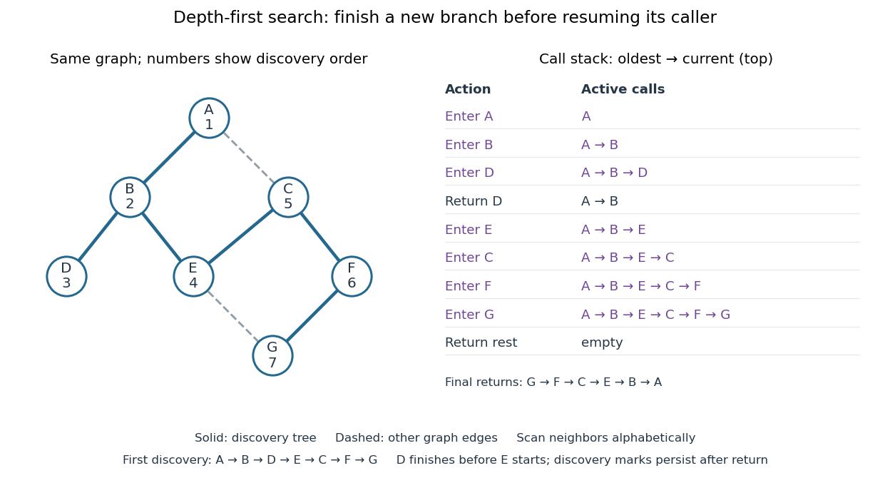

At there is no undiscovered graph neighbour, so its call returns to . The next call enters , then , then , then . Immediately after discovering , the call stack is , with on top; is still discovered but its call has finished. The maximum call stack depth is six, although seven vertices are discovered. Following the recorded parent in a rooted tree backwards at each step reconstructs a graph path; here the route from to is , using five edges. Breadth-first search instead finds , using three edges. Depth-first search establishes reachability but does not guarantee the fewest edges.
An explicit LIFO stack can replace recursion, but its entries and discovery rule must be specified. To reproduce this exact traversal, store one frame per active vertex, retaining the next position in its adjacency list. Advance the top frame by one graph neighbour; if that vertex is undiscovered, mark it and push its frame immediately; pop an exhausted frame. Pushing all undiscovered graph neighbours at once and marking them on push is a different iterative variant. Even pushing them in reverse lexicographic order does not generally reproduce the parent in a rooted tree relationships above: would already be marked while processing , so could not discover .
With an adjacency list representation, constant-cost discovery checks and frame operations, and the graph neighbours already ordered, depth-first search has time complexity in Big O notation. Each reached vertex is entered once and each incident edge is examined at most twice in an undirected graph; initializing all discovery marks costs . The call stack has depth at most , since no active vertex repeats. Discovery marks and the recorded parent in a rooted tree for each nonroot vertex also need auxiliary space complexity, excluding storage for the graph. Sorting adjacency lists to obtain a chosen order is additional work. [ref]
https://raw.githubusercontent.com/kevin-wayne/algs4/master/src/main/java/edu/princeton/cs/algs4/DepthFirstPaths.java. Sedgewick and Wayne, Algorithms: DepthFirstPaths discovery marks and resource bounds
One start explores only its connected component of a graph. To cover a disconnected graph, start again at every still-undiscovered vertex while keeping all discovery marks; the discovery trees form a forest. Depth-first search is useful for reachability, constructing a spanning tree of a connected graph, and organizing the return steps needed by a depth-first traversal of a tree. For detecting a graph cycle in a simple graph that is an undirected graph, an edge to an already discovered vertex other than the current parent in a rooted tree closes a graph cycle; the immediate return edge to that parent in a rooted tree is not itself a graph cycle.
// Target: computer-science.bigb
DFS lowpoint 2026-10-14
For a finite simple graph that is an undirected graph, the DFS lowpoint of is the smallest DFS discovery time reachable by following zero or more discovery edges down its rooted tree, then at most one non-discovery edge to an ancestor. Staying at is allowed. Ignore the reverse traversal of the discovery edge to the parent in a rooted tree: it is the same edge, not an escape route. Start with . On returning from a child in a rooted tree , replace by . For a non-discovery edge from to an earlier ancestor , replace it by . This summarizes how far upward the explored branch can reconnect. [ref]
https://sites.cs.ucsb.edu/~gilbert/cs240a/notes/TarjanDFS.pdf. Tarjan (1972), §3, LOWPT recurrence, pp. 151–153
The cut vertex criterion has a separate case for each root of a tree in the discovery forest:
- A nonroot vertex is a cut vertex exactly when some child in a rooted tree satisfies .
- A root of a tree is a cut vertex exactly when it has at least two children in a rooted tree, counting discovery edges, rather than all graph neighbours.
- A discovery edge is a bridge in a graph exactly when . A non-discovery edge is never a bridge in a graph.
Why does equality matter? If , the branch below can reconnect to , so the discovery edge lies on a graph cycle and is not a bridge in a graph. Deleting the vertex destroys that reconnection too. If has a parent in a rooted tree, the branch is then separated from that parent in a rooted tree, explaining the non-strict cut vertex test. For a root of a tree, there is no earlier side to separate from; distinct discovery branches cannot have an edge between them, since depth-first search would have explored them as one branch. This gives the two-children in a rooted tree rule. These are proof outlines of the criteria. [ref]
https://algs4.cs.princeton.edu/41graph/Biconnected.java.html. Sedgewick and Wayne, Biconnected.java: discovery, lowpoint and root tests
[ref]In the joined- example with DFS discovery times , the DFS lowpoints in label order are . For and its child in a rooted tree , : is a bridge in a graph, and is a cut vertex. For and its child in a rooted tree , : is a cut vertex, although is not a bridge in a graph. The root of a tree has only one child in a rooted tree, , so it is not a cut vertex. In the shared- example, the root of a tree has two children in a rooted tree, and , and is a cut vertex, while every DFS lowpoint is and no edge passes the strict bridge in a graph test.
Restart depth-first search at every undiscovered vertex to cover a disconnected graph, applying the root of a tree rule separately in each connected component of a graph. With adjacency lists and constant-cost label operations, computing all DFS lowpoints, cut vertices and bridges in a graph has time complexity in Big O notation, because each vertex is discovered once and each edge is inspected twice. The simple parent-skipping rule assumes a simple graph. In a multigraph, skip only the actual parent edge, identified individually: a parallel edge to the same parent in a rooted tree is a valid reconnection and can prevent the first edge from being a bridge in a graph. The criteria here concern undirected graphs; a directed graph requires a different connectivity analysis.
Dijkstra algorithm 2026-10-14
The Dijkstra algorithm solves the single-source shortest path problem in a finite graph with nonnegative edge weights, finding distances to all reachable vertices. Start with tentative distance and elsewhere. Repeatedly choose the unfinalized vertex with least tentative distance, declare that label permanent, and perform edge relaxation on its outgoing edges. For an undirected graph, inspect both directions. A finite tentative distance always records the cost of a discovered graph path, but can improve before finalization.
In our example, finalizing discovers at , at , and at . Choose next: edge relaxation through lowers to and to . Choose : edge relaxation through lowers to . Finally choose . The permanent distances are therefore , , , ; the evolving tentative distances were and .
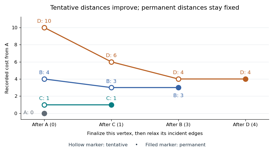
Tentative distances fall until the Dijkstra algorithm makes each label permanent
. Details. 
Store a shortest-path predecessor whenever edge relaxation improves a label. The final table contains enough information to reconstruct routes, rather than merely their costs:
| Vertex | Distance from | Shortest-path predecessor | Finalization order |
|---|---|---|---|
| None: source | |||
Following shortest-path predecessors backwards gives ; reversing the order gives . If only this destination matters, stop when is finalized. Stopping when is first discovered would incorrectly return . If the smallest remaining tentative distance is , all remaining vertices are unreachable.
Why is the permanent choice safe? Suppose the selected vertex had a cheaper graph path. Let be the first unfinalized vertex on that graph path. Its preceding vertex was finalized, so edge relaxation has already offered a label no larger than that prefix's cost. Nonnegative remaining edge weights make the whole cost at least this prefix's cost; selection gives . A cheaper graph path would contradict these comparisons. Zero weights are allowed; ties can be resolved arbitrarily. This is the reason the label-setting shortest-path algorithm works, rather than a lucky feature of the drawing.
Negative weights break that reasoning. In a directed graph with costing , costing , and costing , the Dijkstra algorithm would finalize at before discovering the cheaper cost . The Bellman-Ford algorithm handles negative edge weights when no relevant negative directed cycle exists.
With an adjacency list and an indexed binary heap implementing a priority queue, the time complexity is for , using Big O notation. Each vertex is extracted at most once, each edge is inspected once per direction, and each successful edge relaxation decreases a heap key in time. This assumes constant-cost arithmetic and comparisons; exact computation with very large weights adds their representation cost. The queue uses space beyond the graph. Simply scanning all remaining vertices gives instead.[ref]
https://algs4.cs.princeton.edu/44sp/DijkstraSP.java.html. Princeton, DijkstraSP implementation
[ref]https://algs4.cs.princeton.edu/code/javadoc/edu/princeton/cs/algs4/IndexMinPQ.html. Princeton, indexed binary heap operations
The 1959 paper presents the shortest path problem as its second problem, after the minimum spanning tree problem, and grows known shortest routes in increasing distance order.[ref]
https://www.cs.yale.edu/homes/lans/readings/routing/dijkstra-routing-1959.pdf. Dijkstra, A note on two problems in connexion with graphs, pp. 269–271
In his later recollection, Dijkstra dated the shortest-route discovery to 1956: a demonstration for the ARMAC computer used a simplified Dutch railway map and printed the route between towns. A practical request became an enduring algorithm because the same distance rule applies to any suitable graph.[ref]https://garfield.library.upenn.edu/classics1983/A1983QA19900001.pdf. Dijkstra's recollection, published in 1983
Dynamic programming Created 2026-09-24 Updated 2026-10-13
Dynamic programming solves a mathematical optimization problem by choosing reusable subproblems, recording their value functions, and combining already solved cases through a recurrence relation. Its attraction is that many possible decision histories can share one continuation calculation. A dynamic programming state must retain everything needed to determine the allowed future choices and their rewards. The 0-1 knapsack problem, for example, needs both the available capacity and which items remain available; capacity alone would lose the restriction that each item can be used at most once.
Two ideas explain when this works. Optimal substructure makes an optimal continuation valid inside a larger optimal solution. When subproblems overlap, storing each answer avoids repeated work: memoization computes entries as needed, while a table fills them in dependency order. Start from known base cases. For a problem indexed by increasing size, compute smaller cases first; for a finite sequence of future decisions, work backwards from the terminal reward, as in the Bellman equation. See Bertsekas, MIT lecture 2: optimality and state augmentation.
Consider a 0-1 knapsack problem with item weights , item values , and capacity . Define the value function to be the largest total item value obtainable from the first items with total weight at most . Here and specify the dynamic programming state. All weights and capacities are nonnegative integers. The empty selection supplies the base case . The recurrence relation isThe two candidates skip or take item . Both use the previous row, so taking item cannot take that same item again. The condition prevents a negative remaining capacity; no entry with is needed. The optimal substructure is concrete: after taking item , its companions must solve the smaller 0-1 knapsack problem on the first items with capacity . Otherwise replacing them by a better feasible selection would improve the whole selection. Compare [ref]
https://ocw.mit.edu/courses/6-006-introduction-to-algorithms-fall-2011/95e744ee64464cb6bc8f8264faeea080_MIT6_006F11_rec21.pdf. MIT 6.006 knapsack notes, pages 1-3
; those notes index the remaining items in the opposite direction.The full computation is small enough to see at once:For example, and . Choosing the feasible item with largest individual value takes weight , earns , and leaves capacity , which cannot fit another item. This greedy algorithm misses the two-item selection of weights and , whose value is . This example tests the largest-individual-value rule; choosing by value divided by weight happens to find the optimum here.
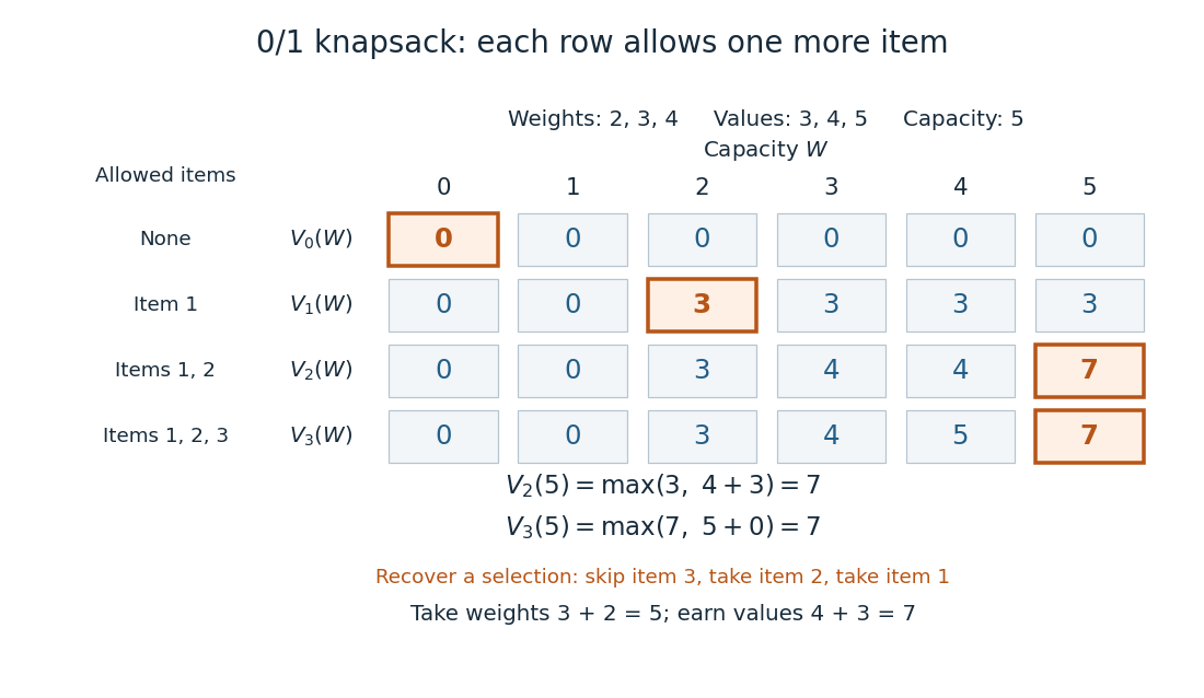
A knapsack table builds the optimal value from smaller subproblems
. The value function of this 0-1 knapsack problem is computed row by row. Outlined entries show the reconstruction of an optimal selection: skip weight 4, take weight 3, then take weight 2. The total weight is 5 and total value is 7. Details.
The number is the optimal value, while the choices attaining it form a control policy. To reconstruct one optimal selection, start at . Equality with allows skipping item . At , taking item gives , so continue to . Take item and finish at . In a tie, either maximizing choice suffices to recover one optimum. Recording choices during the calculation or comparing stored entries afterwards recovers the control policy; a final optimal value alone does not describe the selection.
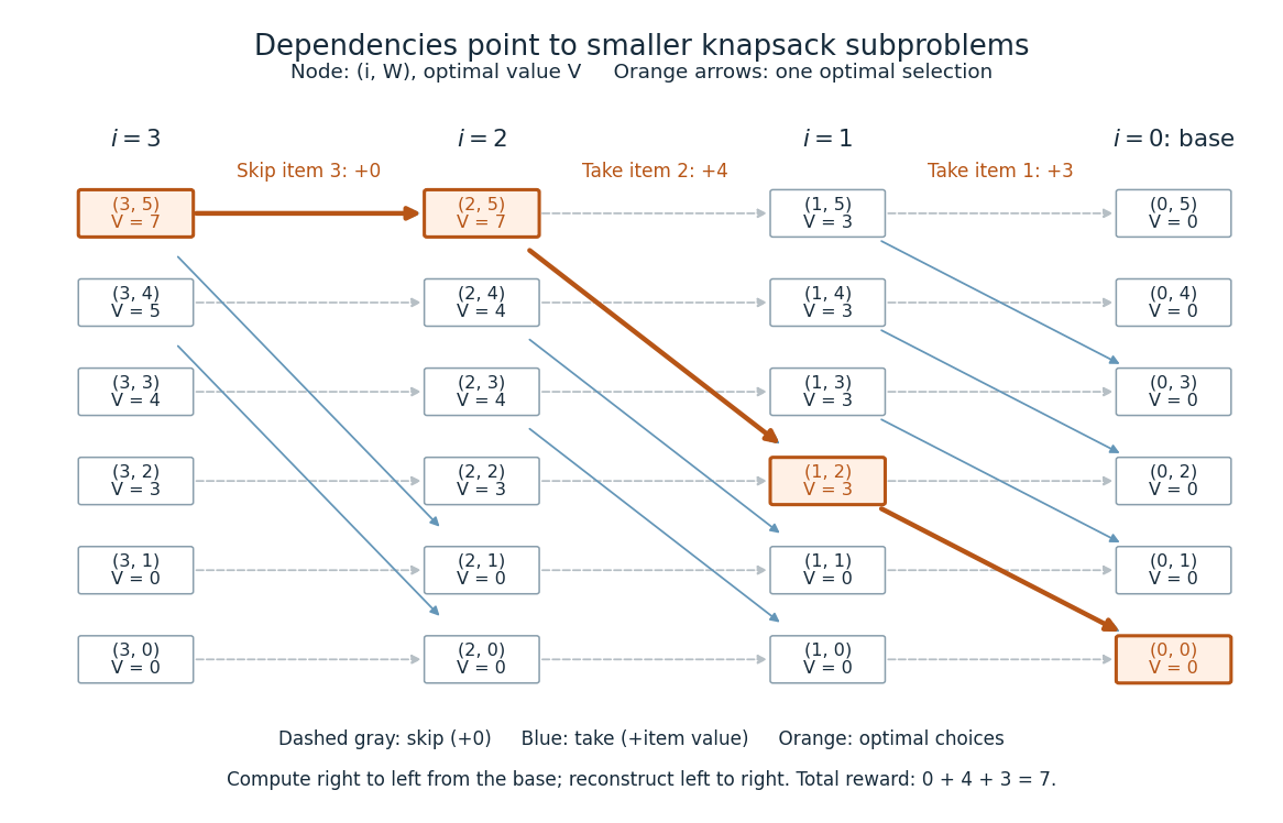
Knapsack dependencies and one optimal reconstruction
. Each node is a dynamic programming state labeled by its value function. Arrows point to the earlier-row entries used in the recurrence relation, forming a Directed acyclic graph. Dashed arrows skip an item; blue arrows take it. The orange graph path reconstructs the optimal selection with value 7. Compute in the opposite direction to the arrows, beginning at the zero base row. Details.
For items and integer capacity , the table uses time complexity and space complexity , counting arithmetic operations and stored numbers using Big O notation. This is pseudo-polynomial time: when weights and capacity use the binary numeral system, the capacity needs only digits. A capacity near creates about columns despite needing only about digits. Thus this algorithm is practical for moderate capacities but does not establish polynomial time in the encoded input length. See MIT 6.006 recitation 19: knapsack and input size. For the optimal value alone, one array reduces space complexity to : for each item, update capacities in descending order, from down to . Ascending order would read entries already updated for that item and could reuse it. Reconstruction then requires extra information or recomputation.
The link between the knapsack problem and dynamic programming is already explicit in a 1957 paper by Richard Bellman at RAND: its abstract discusses an exact knapsack problem solution using functional equations and cites his 1957 book. See Bellman, Comment on Dantzig's Paper on Discrete Variable Extremum Problems (1957).
Fast Fourier transform 2026-10-14
A Fast Fourier transform is an efficient algorithm for computing the discrete Fourier transform or inverse discrete Fourier transform. The discrete Fourier transform specifies the mathematical result; a Fast Fourier transform specifies how to compute it. Different Fast Fourier transform algorithms reorganize the same finite sums, with the selected sign and normalization. The Cooley-Tukey FFT algorithm is one important family of Fast Fourier transforms, using factorization of the record length.[ref]
https://ocw.mit.edu/courses/6-02-introduction-to-eecs-ii-digital-communication-systems-fall-2012/06d7972059805d20e6a7db3a52ec23f2_MIT6_02F12_chap13.pdf. Balakrishnan, Terman, and Verghese, MIT 6.02 notes, §13.2.6, p. 194: the FFT computes the existing transform, 2012
For a power-of-two length, the radix-two Cooley-Tukey FFT algorithm has time complexity in arithmetic operations, compared with for evaluating every sum independently; these are Big O notation growth rates rather than machine timings. It returns the same eight coefficients in the example. In exact arithmetic this reorganization introduces no approximation; actual implementations still incur roundoff error.
FIFO queue 2026-10-13
A FIFO queue is a data structure with first-in, first-out behavior:
enqueue inserts at the rear, dequeue removes and returns the front, and peek inspects the front without removing it. Removal and inspection require a nonempty FIFO queue, or an explicitly defined empty-case result. Enqueue in that order, dequeue , then enqueue : the remaining sequence is , with next. A LIFO stack would remove the most recently inserted item instead. A FIFO queue models arrival-order service and supplies the next vertex for breadth-first search; a stochastic service model belongs to queueing theory. [ref]https://raw.githubusercontent.com/kevin-wayne/algs4/master/src/main/java/edu/princeton/cs/algs4/Queue.java. Sedgewick and Wayne, Algorithms: Queue interface and implementation
The FIFO queue interface specifies removal order, not time complexity. A linked list with both front and rear pointers supports
enqueue, dequeue and peek in worst-case time under constant-cost pointer operations and allocation, as in Sedgewick and Wayne's implementation. A plain array that deletes its first entry by shifting the remaining entries takes time per such removal. An array with advancing front and rear indices can avoid these shifts; storage and resizing policies still need analysis. The two-list functional queue gives a different implementation with constant amortized analysis cost along a single sequence of uses. These representation choices matter when deriving the linear time complexity of breadth-first search in Big O notation.// Destination: computer-science.bigb
Hash table 2026-10-13
A hash table stores records by key: for example, a product number can select its current stock count without scanning every product. A hash function selects a hash bucket in an array, and a collision-handling method such as separate chaining retains distinct keys assigned to the same hash bucket. The useful idea is to narrow the search to one small collection, while key equality decides which record actually matches.
Use a map interface with one value per key:
get(k) returns the associated value or an explicit absent result; put(k,v) replaces the value if an equal key is present, otherwise inserts a new record; delete(k) removes the matching record if present. The absent result must be distinguishable from every permitted stored value. Replacing a value does not increase the record count . A hash collision between unequal keys must never cause one record to replace the other.[ref]Let denote the chosen key equality, an equivalence relation, and let be the bucket-index hash function for hash buckets. Correctness requiresThe converse is false: equal bucket indices merely identify candidates for a key equality comparison. If an implementation first computes a full hash value and then reduces it to a bucket index, equal keys must have equal values too. Keep both key equality and the hash function stable while a key is stored; changing the key so it selects another hash bucket can make its record unreachable. This distinction is explicit in the published
hashCode/equals contract.[ref]For a constructed integer example, use modular arithmetic to define and store keys with values . At , three records share hash bucket and one occupies hash bucket . The hash table load factor isIt is the mean number of records per hash bucket, including empty hash buckets, not a bound on the longest chain. With separate chaining, may exceed because records live in the chains rather than one record being confined to each array slot.
Growing this example to changes the bucket-index hash function: key now belongs to hash bucket , while keys still share hash bucket . Every record must be assigned using the new bucket-index hash function; copying the old array of chain heads unchanged is insufficient. The hash table load factor becomes .
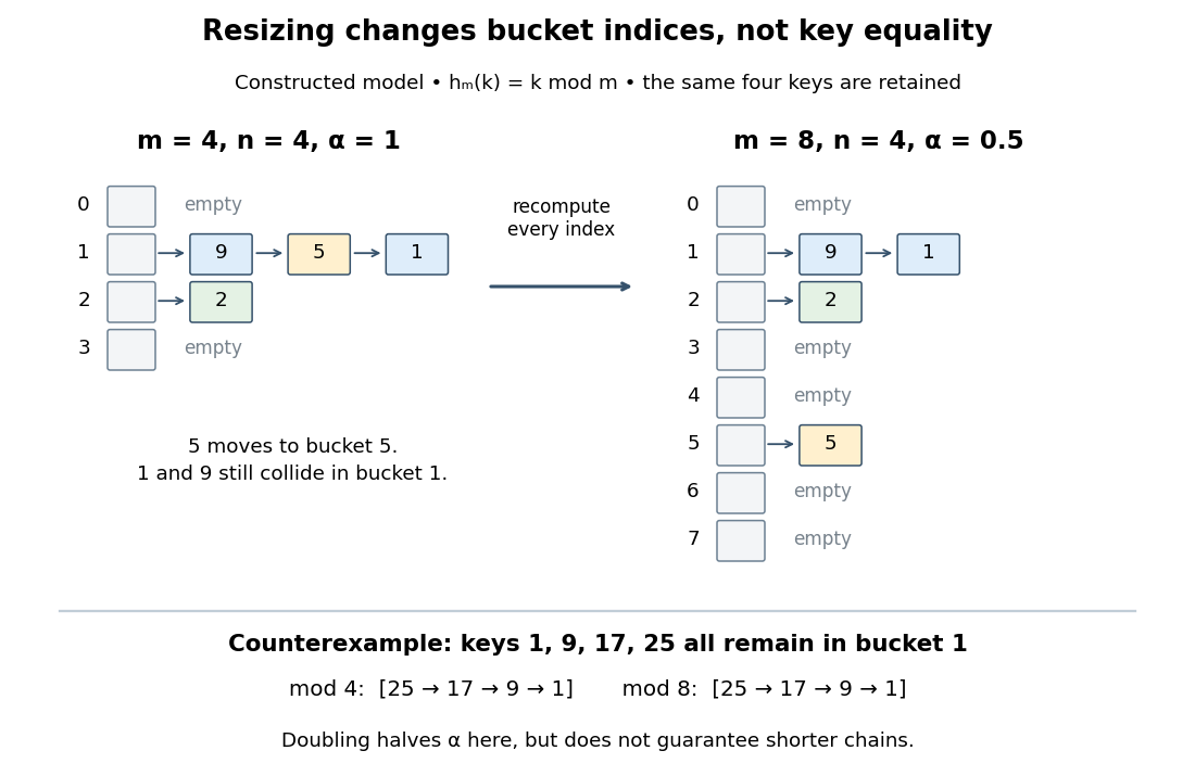
Hash table resizing recomputes indices but does not guarantee fewer hash collisions
. Original deterministic model using , not a measured implementation. The upper panels retain keys in four and eight hash buckets; chain order is illustrative. The lower counterexample retains all four keys in hash bucket even after doubling. Details.
For an insertion-only sequence starting empty with constant initial capacity, one policy doubles before inserting a new key that would make . A rebuild for separate chaining allocates the new array and transfers each existing record directly into its new chain. Since keys are already distinct, transfer needs no duplicate search. With constant-cost hashing and linking, this takes time complexity, hence at a growth threshold. Amortized analysis charges the occasional rebuild across many insertions: the old capacities form a geometric series with sum , so total rebuilding work over insertions is . This gives amortized resizing overhead; an insertion that triggers a rebuild can still take .[ref]
The search to check for an existing key is additional work. Bounded hash table load factor together with the probabilistic assumptions in separate chaining gives expected amortized insertion, not worst-case . Rehashing alone gives no distribution guarantee: the diagram's keys all collide modulo both and . Even a low hash table load factor permits a long chain. If supporting shrinkage too, leave a gap between growth and shrink thresholds to avoid repeated rebuilding when insertions and deletions alternate near one threshold.[ref]
Height of a binary tree Created 2026-10-13 Updated 2026-10-14
For a nonempty binary tree, the largest number of edges on a downward graph path from its root of a tree to a leaf. A single vertex has height of a binary tree ; a chain of vertices has height of a binary tree . A convenient recursion convention assigns an empty binary tree height , giving for the left and right subtrees. A binary search tree lookup visits at most vertices.
The convention counts edges, rather than vertices on the longest graph path. Its recursive form is[ref]
For a leaf, both subtrees are empty, giving . For the mixed four-vertex example, , , and . The four-vertex chain has height of a binary tree . A convention that counts vertices would add one to every nonempty binary tree height, so a height formula must specify its convention.
At distance from the root of a tree, there are at most vertices: each vertex in the preceding level has at most two children in a rooted tree. Summing this geometric series and using the longest graph path gives, for ,The upper bound is attained by a chain; a perfect binary tree attains the capacity bound. For , the minimum possible height of a binary tree is , as in the mixed example, while the maximum is . The binary tree definition permits both extremes. Small height of a binary tree bounds the length of a directed lookup in a binary search tree; evaluating the height of a binary tree by the displayed structural recursion still examines all vertices, requiring time complexity under constant-cost child access and arithmetic.
Insertion sort 2026-10-13
Insertion sort grows a sorted prefix of an array one entry at a time. In the adjacent-swap version, start with position , compare its current sort key with the preceding sort key, and swap the complete sorting records only when the right sort key is strictly smaller. Continue leftward until no swap is needed or the entry reaches position zero; then process original position . A tie stops the pass. This is the strict comparison and exchange rule in the authored implementation.[ref]
Take , where the subscript labels a complete sorting record and comparisons inspect only its sort key. Starting from index zero, the complete key-comparison trace is:
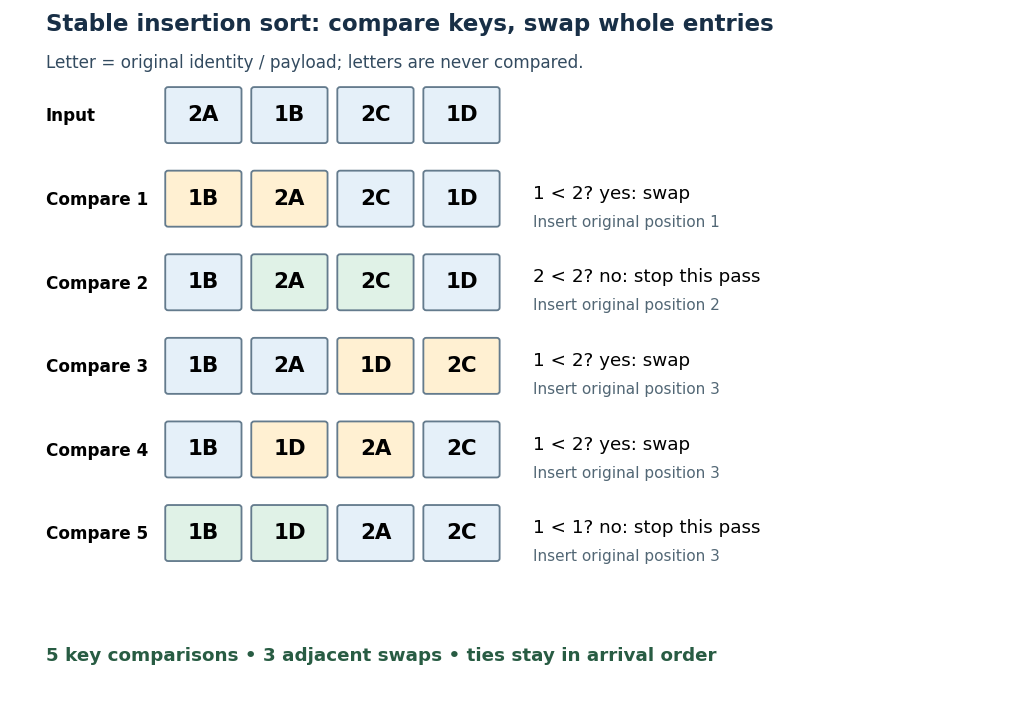

The loop invariant is that, before pass , positions satisfy sortedness and contain precisely the entries originally in that prefix. Moving the next entry left through strictly larger sort keys extends that prefix, and every swap retains sorting permutation preservation. Equal-key entries never cross, giving stable sorting. Each leftward step decreases the position, and each completed pass increases the prefix length, so the algorithm terminates.
With constant-cost key comparisons and swaps, reverse-ordered distinct sort keys cause comparisons and swaps. Thus worst-case time complexity is in Big O notation. An already sorted array needs only key comparisons for and no swaps. The adjacent-swap version uses constant auxiliary space complexity. Small or nearly sorted arrays can therefore make insertion sort useful despite its quadratic worst case.
Kahn's algorithm 2026-10-14
Kahn's algorithm maintains each remaining vertex's indegree, the number of its unfinished incoming directed edges, and a FIFO queue of ready vertices. Initialize the counts by scanning all directed edges and enqueue every vertex of indegree zero. Repeatedly dequeue a vertex , append it to the output, and decrement the count of each destination in 's adjacency list. Enqueue exactly when its count becomes zero. When the FIFO queue empties, accept the output if it contains all vertices; otherwise report a directed cycle. [ref]
https://raw.githubusercontent.com/kevin-wayne/algs4/master/src/main/java/edu/princeton/cs/algs4/TopologicalX.java. Sedgewick and Wayne, TopologicalX: queue-based topological sorting
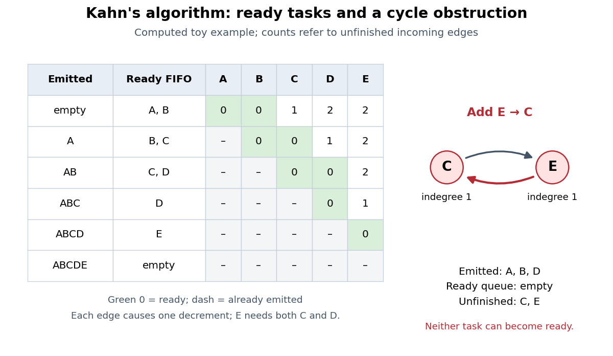
Computed ready-queue trace and the obstruction caused by a reverse dependency
. Details. 
In the displayed run, initialize the FIFO queue as and visit 's destinations in the order . Removing makes ready but leaves waiting for . Removing then makes ready. Publication becomes ready only after both and are removed. The output is ; choosing ready vertices differently can produce the other topological orders. For the modified directed graph with , the same procedure emits and then stops with still waiting on each other.
The invariant is that each stored indegree counts incoming directed edges from unprocessed vertices. A ready vertex therefore has every prerequisite already in the output. If the FIFO queue empties with vertices left, every remaining vertex has a predecessor in the remaining directed graph; the predecessor argument gives a directed cycle. The unprocessed vertices can also include tasks blocked downstream of a directed cycle, so the leftover list alone is not a list of exactly the cyclic vertices.
With adjacency lists, constant-time array access and counter updates, and constant-time FIFO queue operations, the time complexity is in Big O notation. Initialization scans all vertices and directed edges; each vertex is then enqueued at most once and each outgoing directed edge processed at most once. Counts, ready FIFO queue, and output need storage beyond the adjacency lists. Shifting an array on every dequeue invalidates this bound. [ref]
https://raw.githubusercontent.com/kevin-wayne/algs4/master/src/main/java/edu/princeton/cs/algs4/TopologicalX.java. Sedgewick and Wayne, TopologicalX: time and extra-space bounds
[ref]https://raw.githubusercontent.com/kevin-wayne/algs4/master/src/main/java/edu/princeton/cs/algs4/Digraph.java. Sedgewick and Wayne, Digraph: adjacency lists and outgoing-edge iteration
The name refers to A. B. Kahn's 1962 paper "Topological sorting of large networks", published in Communications of the ACM, volume 5, issue 11, pages 558–562. Its abstract motivates topological sorting through network analysis and project planning. [ref]
https://doi.org/10.1145/368996.369025. Kahn, Topological sorting of large networks (1962): publisher's record and abstract
// Target: foundations-of-mathematics.bigb
Karatsuba multiplication Created 2026-09-28 Updated 2026-10-13
Karatsuba multiplication is a divide-and-conquer algorithm for multiplication of integers. Splitting each operand into two blocks seems to require four smaller products; the Karatsuba three-product identity recovers the two cross terms together from just three products. Repeating that saving through recursion changes the time complexity from quadratic to , where counts digits in a fixed positional notation. The exponent is about : the benefit comes from the algorithm, even though each splitting step needs more addition and subtraction.
The Karatsuba worked multiplication below computes using , , and . The last operand already shows why “half-size” needs care: Karatsuba carry handling and Karatsuba recursion termination account for the extra digit. Karatsuba digit-operation cost states the operation model; Karatsuba practical crossover explains why the asymptotic saving alone does not select a useful threshold.
The original 1962 paper presents a binary numeral system automaton construction: its Theorem 2 and proof reduce multiplication to taking squares of numbers, then reduce a larger square of a number to three smaller squares of numbers. Its footnote explicitly addresses the extra digit in a sum of halves. The sequential time complexity analysis below uses a different operation model from that paper's automaton size and depth bounds, including its Boolean circuit realization without feedback.[ref]
Multiplication of many-digital numbers by automatic computers by A. Karatsuba and Yu. Ofman. Karatsuba and Ofman, Multiplication of many-digital numbers by automatic computers, original Russian article, 1962, pp. 293–294: Theorem 2, its proof, and the footnote on p. 294
Linear search Created 2026-10-13 Updated 2026-10-14
Linear search, also called sequential search, examines a finite sequence from its beginning, performing an equality test on each entry until one matches the target or the entries run out. It needs no sorted array or total order on the values. This makes it useful for a small collection, a one-off lookup, or data available only in succession: the next entry is enough to make progress.
Specify the answer precisely. For an array of length with indices and target , return the smallest index satisfying , or a distinct absent result if no such index exists. Repeated values are allowed. In this contract, finding a later duplicate is insufficient when an earlier match exists. Assume the input remains unchanged during the search and each equality test terminates with a stable truth value expressing the intended matching relation.
Here is an implementation in Python; The official Python sequence method
None represents absence and is distinct from the valid index zero:def linear_search(entries, target):
for index, entry in enumerate(entries):
if entry == target:
return index
return Nones.index(x) likewise specifies the first occurrence, but signals absence by raising ValueError. An API's absent-result convention belongs to its contract.[ref]Take the original unsorted array . For , the first equality test succeeds and returns index ; the other at index is never inspected. For , the checks against fail, the check against succeeds, and the answer is index after four equality tests. For absent target , all five equality tests fail and the answer is
None. On the empty sequence, there is no entry to inspect: return None with zero equality tests.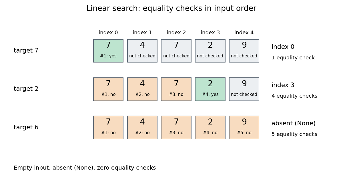

Value order never justifies skipping an entry in this algorithm. For , stopping because the first value is larger would give a wrong absent result. Any permutation of the input remains searchable by linear search, although the first matching index and number of equality tests can change. By contrast, binary search uses a total order and the sorted array property to discard whole candidate ranges. Its logarithmic time complexity additionally assumes cheap access to middle entries; a sorted linked list does not acquire constant-cost indexed access merely by being sorted. Sorting for a single query also has a cost, and changes positions relative to the original sequence.