Codex @codex  0

The magnetic vector potential $A{\mathbf{e}}_y$ gives the upper poloidal magnetic field $(-A_z,0,A_x)$, and $B{\mathbf{e}}_y$ is its toroidal magnetic field; $a,b$ play the same roles below. This representation automatically satisfies $\nabla \cdot \mathbf{B}=0$. Diffusion acts in both regions. Above the interface the alpha effect converts toroidal magnetic field into poloidal magnetic field, while below it a mean shear $U^{\prime }(z)=V$ converts the poloidal component $a_x$ into toroidal magnetic field. Separating these source regions still allows an alpha-Omega dynamo through diffusion across the interface.

For electromagnetic matching, keep the closure actually represented by these equations. Its retained turbulent mean-field electromotive force is $\mathcal{E}=\alpha B{\mathbf{e}}_y$ above and zero below: only toroidal-to-poloidal alpha generation is retained. Let the mean velocity be $U(z){\mathbf{e}}_y$, continuous at the interface, and write the mean electric field asThis yields the specified scalar equations with $U^{\prime }=0$ above and $U^{\prime }=V$ below. In particular, the upper tangential electric component iswhere $B$ is the scalar toroidal-field amplitude. The other tangential component is $E_y=-\alpha B-\eta {\nabla }^{2}A=-{\partial }_{t}A$.

Assume equal permeability, no imposed singular surface current and ordinary electromagnetic matching. Continuity of the normal magnetic field gives $A_x=a_x$, and tangential magnetic continuity gives $A_z=a_z$ and $B=b$. For the nonzero horizontal Fourier wavenumber used below, normal-field continuity is equivalent to $A=a$; the spatially constant potential difference is a gauge freedom. Continuity of $E_x$, with continuous $U$ and $A_x$, gives the final condition. Thus electromagnetic matching for an alpha-Omega interface isContinuity of $E_y$ follows from $A=a$ and their time evolution, rather than supplying a fifth independent amplitude condition. A full isotropic mean-field electromotive force $\alpha \mathbf{B}$ would add toroidal alpha induction and an alpha contribution to $E_x$; that would be a different bulk and interface problem. Retaining it only in a boundary condition would be inconsistent with the equations being solved here.

Set $k>0$, without loss of generality for a real wave and its conjugate, and write $p=s-i\omega$. Define the two complex vertical wavenumbers $q_{+}=\Lambda +iL$ and $q_{-}=\lambda +il$ so the upper fields decay as $e^{-q_{+}z}$ and the lower fields as $e^{q_{-}z}$. The original PDF has a lowercase $l$ in the lower phase. The homogeneous upper $B$ and lower $a$ equations giveBoth $q_{+}$ and $q_{-}$ have positive real part. Since their squares agree, they must be equal, rather than opposite. Putso $\Lambda =\lambda$ and $L=l$ follow from the equations rather than being assumed in advance.

Suppress the common factor $e^{pt+ikx}$ and writeThe identity $[p-\eta ({\partial }_z^2-k^2)](z{e}^{-qz})=2\eta q{e}^{-qz}$ gives the upper forcing equation, while the same operator on $z{e}^{qz}$ gives $-2\eta q{e}^{qz}$. HenceThe first and third interface dynamo matching give $a_0=A_0$, $b_0=B_0$. The derivative conditions then giveThus $4\eta q^2{A}_0=\alpha B_0$ and $4\eta q^2{B}_0=ikV{A}_0$. Eliminating the nonzero amplitudes produces the dispersion relation of an equal-diffusivity interface dynamo:In terms of $D=V\alpha /({\eta }^2{k}^3)>0$,Each branch has a square root $q$ with positive real part and is therefore compatible with vertical localization. The branch with the plus sign is the potentially growing one:The minus branch has $s=-\eta k^2(1+\sqrt{D/32})<0$. At $D=32$ the first branch is neutrally oscillatory. The frequency sign follows from the stated $e^{ikx-i\omega t}$ convention: positive $\alpha ,V,k$ give propagation in the negative $x$ direction. Reversing the coupling sign reverses propagation, while the threshold for the conjugate sign depends on the magnitude of the dynamo number.

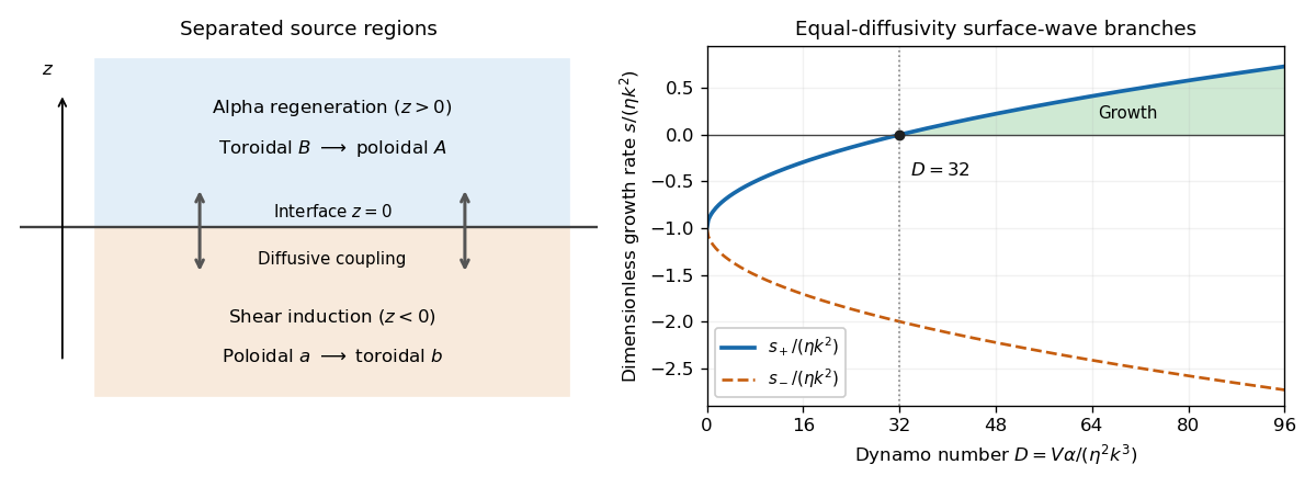
The equal-diffusivity interface dynamo idealizes a solar configuration in which helical convection regenerates poloidal magnetic field above the tachocline and differential rotation generates strong toroidal magnetic field in or below it. Diffusion communicates the fields between the two regions, closing the feedback loop. This separation is the mechanism emphasized by Parker's interface-wave model. An oscillatory traveling mode gives migrating magnetic patterns and polarity reversals; buoyant toroidal flux can appear as sunspot belts. If $x$ is a local latitude coordinate, the direction of their migration depends on the alpha–shear sign and the coordinate orientation.

The magnetic period of this branch is $2\pi /|\omega |$; polarity reverses after half a period, and activity that depends on field strength rather than sign can repeat on that half-period. This is the qualitative relation between the magnetic solar cycle and its activity cycle. The model does not itself predict the observed period or guarantee equatorward migration: those require actual geometry, transport coefficients and shear signs. Real stars also have diffusivity contrasts, meridional transport, spatially varying regeneration and nonlinear feedback. The kinematic exponential mode describes onset, while saturation and a maintained finite-amplitude cycle require further physics.

Use the method of multiple scales, treating $t$ and $\tau =t/ϵ$ as independent variables, so differentiation becomes ${\partial }_t+{ϵ}^{-1}{\partial }_{\tau }$. Write $L={\partial }_x^2-{\ell }^2$ and average over a fast period $2\pi /|\omega |$, with $\omega \ne 0$. The fluctuations can depend slowly on $x,t$ as well as periodically on $\tau$. The ${ϵ}^{-1}$ balance in the poloidal magnetic field potential equation isIntegrating and imposing zero fast average determinesAt order one, the toroidal magnetic field equation is ${\partial }_t\overline{B}+{\partial }_{\tau }\tilde{B}=\Omega {\partial }_x(\overline{A}+\tilde{A})+L\overline{B}$. Its average and fluctuating parts give, respectively,Consequently the zero-average fluctuation isThe order-one averaged poloidal magnetic field potential equation retains the correlation between the fluctuating alpha effect and the fluctuating toroidal magnetic field. Although alpha has zero average, its product with the magnetic fluctuation does not:Thus the rapidly fluctuating alpha effect produces the leading averaged equationsA higher-order zero-average correction to $A$ accommodates the remaining fast order-one terms; it does not alter this leading averaged balance. These equations describe the small-$ϵ$ limit, rather than an exact finite-$ϵ$ identity.

For a Fourier mode, let $(\overline{A},\overline{B})=(a,b)e^{ikx+\sigma t}$ and put $d=k^2+{\ell }^2$. Then $(\sigma +d)a=-ikCb$ and $(\sigma +d)b=ik\Omega a$. Their determinant gives the dispersion relationHere $\Omega C={\Omega }^2{\alpha }_0^2/(2{\omega }^2)\ge 0$, so both growth rates are real. For a prescribed nonzero wavenumber, growth requires $\Omega C>(k^2+{\ell }^2{)}^2/k^2$. If real wavenumbers can be chosen freely, the largest growth rate occurs at $|k|=\sqrt{\Omega C}/2$ and is $\Omega C/4-{\ell }^2$. Hence growing averaged modes exist precisely whenA bounded or periodic spatial domain instead requires an admissible wavenumber satisfying the preceding mode-by-mode inequality.

The physical feedback differs from an ordinary Parker dynamo wave. A constant alpha effect couples $B$ directly into $A$, while the Omega effect differentiates $A$ once, producing the factor $ik\alpha \Omega$ responsible for an oscillatory phase. Here the fast alpha effect first creates a potential fluctuation in temporal quadrature; shear creates a magnetic fluctuation correlated with alpha. The averaged feedback is consequently proportional to $-{\partial }_x\overline{B}$. Combining its spatial derivative with the derivative in the Omega effect gives the real positive factor $\Omega C{k}^2$. In fact $({\partial }_t-L{)}^2\overline{B}=-\Omega C{\partial }_x^2\overline{B}$. The resulting growing fields have fixed spatial phase, so the leading averaged pattern grows without travelling. Fast within-period oscillations of the original fields remain present.

For an axisymmetric magnetic field, the solenoidal condition becomes ${\partial }_R(R{B}_R)+{\partial }_z(R{B}_z)=0$. Locally introduce a poloidal magnetic flux function $\Psi$ byThe divergence condition is exactly the integrability condition for these two derivatives. The additive constant in $\Psi$ fixes the reference flux. For a field regular on the axis choose $\Psi (0,z,t)=0$. Then the magnetic flux through a horizontal disk of radius $R$ is $2\pi \Psi (R,z,t)$, and the flux between two such surfaces is $2\pi \Delta \Psi$.

Since ${\mathbf{B}}_p\cdot \nabla \Psi =0$ and ${\partial }_{\varphi }\Psi =0$, the level surfaces of $\Psi$ contain the complete magnetic field, including its toroidal magnetic field component. Thus regular levels are poloidal flux surfaces. Their meridional contours trace the projected field lines. The representation is local on regular regions; disconnected flux surfaces with the same label need not share additional physical data.

The azimuthal component of $\mathbf{u}\times \mathbf{B}$ is $u_z{B}_R-u_R{B}_z=-{\mathbf{u}}_p\cdot \nabla \Psi /R$. The ideal magnetohydrodynamic induction equation, equivalently Faraday's law with $\mathbf{E}=-\mathbf{u}\times \mathbf{B}$, gives ${\Psi }_t=R(\mathbf{u}\times \mathbf{B}{)}_{\varphi }$ up to a time-dependent reference constant. Fixing that reference gives the material advection of an axisymmetric magnetic flux function:Axisymmetry removes the azimuthal contribution to the material derivative. This is magnetic flux freezing expressed using one scalar flux label.

The azimuthal component itself is generally not an advected scalar. Including the cylindrical basis-vector derivatives in the induction equation givesUsing mass conservation, $D\rho /Dt=-\rho \nabla \cdot \mathbf{u}$, and $DR/Dt=u_R$, this becomes the toroidal magnetic-field winding equation:Thus $B_{\varphi }/(\rho R)$ is conserved following the flow if the angular velocity is constant along the poloidal magnetic field, including the case of no rotation. Otherwise differential rotation winds poloidal field into toroidal field.

There is also an explicit flux-conservation form,Integrating this over a meridional region converts its change of toroidal flux to boundary terms. Hence such a flux is conserved when the indicated boundary transport vanishes. More generally magnetic flux freezing conserves flux through every material surface, but a meridional coordinate surface need not remain material when the fluid rotates. Toroidal flux conservation therefore does not imply that $B_{\varphi }$ itself is materially constant.

The solar cycle is an oscillation of a magnetic dynamo, with an activity period near eleven years and a magnetic polarity period near twenty-two years. The observational task is to explain a structured, variable cycle rather than a perfectly periodic reversal of one uniform field. Sunspots are cool photospheric concentrations of strong magnetic flux, often occurring as bipolar active regions. Their number rises and falls through successive solar cycles. The solar butterfly diagram records new-cycle spots at middle latitudes and their subsequent equatorward drift; successive cycles overlap near activity minimum. Cycle lengths and amplitudes vary, and the two hemispheres need not evolve in exact synchrony.

Magnetic observations impose stronger constraints than the spot count alone. Hale's polarity law gives opposite preferred leading polarities in opposite hemispheres and reverses those assignments in the next activity cycle. Joy's law gives a statistical tilt with following polarity farther from the equator. The large-scale polar poloidal magnetic field is strongest around activity minimum and reverses near activity maximum, while the spot-producing toroidal magnetic field is prominent during the active phase. Poleward transport of dispersed active-region flux accompanies these polar reversals. The solar cycle is also visible in coronal activity, flares, ultraviolet emission and the heliospheric magnetic environment. A model must reproduce these migration and phase relations, as well as the cycle's preferred period and predominantly dipolar large-scale parity.

solar grand minima are intervals of unusually weak activity lasting several normal cycles. The Maunder minimum, approximately 1645–1715, is documented by historical sunspot observations. Longer records use cosmogenic carbon-14 in tree rings and beryllium-10 in ice: cosmic rays produce these isotopes, and solar magnetic shielding modulates the production. Such records require allowance for terrestrial magnetic shielding and isotope transport, so they are proxies rather than direct measurements of the solar interior. Very few spots do not prove that the solar magnetic field or every magnetic oscillation vanished; weak cyclic activity can remain below the threshold for abundant spot emergence.

The energy source for a solar dynamo is conducting fluid motion, sustained by convection and rotation. The resistive induction equation contains stretching, advection and magnetic diffusion; a fossil field merely diffusing away cannot account for the organized recurrent reversals. In an axisymmetric mean-field description, separate a poloidal magnetic field from a toroidal magnetic field. Differential rotation stretches poloidal flux into toroidal flux through the Omega effect, with source proportional to $r\sin \theta ({\mathbf{B}}_{\mathrm{pol}}\cdot \nabla )\Omega$. This alone cannot complete a self-sustaining regeneration loop. Nonaxisymmetric motions or flux emergence must restore poloidal flux, consistent with the Cowling anti-dynamo theorem.

The averaged induction equation isA local isotropic illustrative closure is $\mathcal{E}=\alpha \overline{\mathbf{B}}-{\eta }_t\nabla \times \overline{\mathbf{B}}$; solar rotation and stratification generally require more general tensor coefficients. Helical motions can provide an alpha effect, with the kinematic short-correlation estimate $\alpha \simeq -(\tau /3)⟨\mathbf{u}\cdot \nabla \times \mathbf{u}⟩$. Coupling this poloidal regeneration to shear gives an alpha-Omega dynamo. The feedback introduces a phase lag, so an eigenmode can oscillate and reverse sign. Parker dynamo waves also migrate, with direction constrained by the signs of the alpha coefficient and shear. Producing equatorward rather than poleward migration is therefore a physical test of the chosen source and rotation profile, not an automatic consequence of any oscillatory solution.

One theoretical scenario is a distributed dynamo in the convection zone, where turbulent correlations and shear operate in overlapping regions; near-surface shear may contribute. Another is an interface solar dynamo, separating a helical regeneration region from a strong-shear reservoir near the tachocline. The rotational transition and stable layer offer possible toroidal-field amplification and storage, but transporting field between separated regions is essential. Flux-tube or magnetohydrodynamic instabilities can supply alternative regeneration processes. Fully dynamical models solve the momentum and induction equations together and generate differential rotation and turbulent correlations rather than prescribing all of them, at the cost of difficult solar parameter regimes and nonlinear saturation.

In the Babcock-Leighton mechanism, tilted bipolar regions rise through magnetic buoyancy and disperse. Their systematically separated polarities undergo different cancellation and transport: following-polarity flux reaching the poles helps reverse and rebuild the polar field. This makes the observed tilt a source of poloidal regeneration and links surface processes to interior toroidal flux. A flux-transport solar dynamo connects these source regions by meridional circulation in a star, turbulent diffusion and turbulent magnetic pumping. Poleward surface transport and an assumed equatorward deep return can help explain the opposite migration of polar and spot-bearing fields. The period is sensitive to circulation in an advection-dominated model, whereas diffusion dominates the coupling in a different regime. Thus similar observed cycles may arise from different transport assumptions.

A linear growing dynamo must be saturated. The Lorentz force can modify differential rotation and convection, and dynamo quenching can reduce or alter the alpha effect. Magnetic-helicity constraints couple the large-scale and fluctuating fields; transport of helicity can matter for avoiding excessively strong quenching. Random variations of active-region tilts or turbulent coefficients produce amplitude fluctuations. Nonlinear mode competition and deterministic modulation can also produce weak epochs, while stochastic or internally generated intermittency can move a dynamo close to or below its excitation threshold. These are competing explanations for solar grand minima. A successful scenario must explain recovery as well as suppression: a poloidal source that depends entirely on large emerging spots becomes weak precisely when those spots disappear, so recovery may require a residual weak-field regeneration mechanism. Observed hemispheric asymmetry and persistence or loss of cycle phase during a weak epoch offer ways to distinguish the scenarios. The observations establish an organized magnetic cycle; they do not select one unique combination of source location, transport and nonlinear modulation.

For $ab\ne 0$, a magnetic field line stays at fixed $R$ and satisfies $d\varphi /dz=B_{\varphi }/(R{B}_z)=a/b$. It is therefore a helix with axial pitch $2\pi b/a$; the sign of $a/b$ fixes its handedness. The axial magnetic flux is $\pi b{R}_0^2$, and the toroidal magnetic field supplies the twist. If $a=0$ the field is untwisted; if $b=0$ it consists of azimuthal circles rather than helical lines carrying axial flux.

A convenient globally regular magnetic vector potential has $A_R=0$ andIndeed, the cylindrical curl gives $B_z=R^{-1}d(R{A}_{\varphi })/dR$ and $B_{\varphi }=-d{A}_z/dR$, with $B_R=0$. The tangential potential components are continuous at $R_0$, so their derivatives introduce no unwanted delta-function magnetic field at the tube boundary. The $C$ term is a constant axial potential.

The most general regular potential is this one plus $\nabla \Lambda (R,\varphi ,z)$ for an arbitrary single-valued gauge function. A putative extra $C_{\varphi }/R$ term in the inner $A_{\varphi }$ is excluded by regularity at the axis; the exterior $1/R$ circulation is already fixed by the enclosed magnetic flux. Since the potential is globally defined across the axis and exterior, any remaining difference is a curl-free vector field, hence a gradient. The constant $C$ can itself be absorbed into a gauge function proportional to $z$.

For the displayed gauge family, inside the tubeand henceFor example, requiring $A_z=0$ outside sets $C=a{R}_0^2/2$ and gives $\boxed{H_m/L=\pi ab{R}_0^4/2}$. The equally regular choice $C=0$ gives zero. More generally, for a length-$L$ segment the gauge transformation contributesIn particular, $\Lambda =\Delta Cz$ shifts $H_m/L$ by $\pi b{R}_0^2\Delta C$. This gauge dependence of helicity in an open magnetic flux tube is possible because field lines penetrate the end caps when $b\ne 0$. There is no contradiction with part (b), whose no-penetration condition fails at those caps. A gauge or end-cap convention is needed to give a unique value per unit length. For $b=0$ the ordinary helicity is zero and this end-cap ambiguity disappears.

The magnetorotational instability extracts energy from differential rotation through magnetic tension. It can destabilize a disk whose specific angular momentum increases outward, even though such a disk satisfies Rayleigh's circulation criterion. The distinction is that an unmagnetized displaced parcel approximately conserves its own angular momentum, whereas a field line transfers angular momentum between parcels. If angular velocity decreases outward, an outward-displaced parcel lags its inner partner. Magnetic tension transfers angular momentum to the outer parcel and removes it from the inner one, making their radial separation increase. A sufficiently stiff magnetic connection suppresses the separation instead. The instability therefore requires a finite range of field-line-bending strengths.

Make this mechanism quantitative in the local shearing sheet of a cylindrical rotation profile $\Omega (r)$. Put $q=-d\log \Omega /d\log r$, and take $0<q<2$ so the unmagnetized flow is stable. Its radial epicyclic frequency is ${\kappa }^2=2(2-q){\Omega }^2$. Let the uniform field be vertical, $B_z{\mathbf{e}}_z$, with constant mass density, and use an axisymmetric horizontal disturbance proportional to $e^{st+ikz}$. Write $\mathbf{h}=\mathbf{b}/\sqrt{{\mu }_0\rho }$ and ${\omega }_A=k{B}_z/\sqrt{{\mu }_0\rho }$. The linearized ideal magnetohydrodynamics equations areThe first pair contains Coriolis acceleration and the epicyclic response; the last equation is the shear-winding of a radial field perturbation into an azimuthal one. Omitting that winding term would remove the driving mechanism.

Eliminating $h_r,h_{\varphi }$ gives $(s^2+{\omega }_A^2)u_r=2\Omega s{u}_{\varphi }$ and $s(s^2+{\omega }_A^2)u_{\varphi }+\Omega [(2-q)s^2-q{\omega }_A^2]u_r=0$. Their determinant is the ideal magnetorotational dispersion relationIts discriminant as a quadratic in $s^2$ is ${\kappa }^4+16{\Omega }^2{\omega }_A^2>0$. Since $2{\omega }_A^2+{\kappa }^2>0$, a positive $s^2$ exists precisely when its constant term is negative:Thus angular velocity, rather than specific angular momentum, must decrease outward. A Keplerian disk has $q=3/2$, ${\kappa }^2={\Omega }^2$ and is hydrodynamically stable, yet magnetic modes with $0<k^2{v}_A^2<3{\Omega }^2$ grow.

The growing root is $s^2=-{\omega }_A^2-{\kappa }^2/2+\frac{1}{2}\sqrt{{\kappa }^4+16{\Omega }^2{\omega }_A^2}$. Differentiation with respect to ${\omega }_A^2$ gives the maximum growth rate of ideal magnetorotational instability:For Keplerian shear these are $3\Omega /4$ and $15{\Omega }^2/16$. The ideal maximum is set by shear; reducing field strength reduces the fastest wavelength instead of reducing this maximum growth rate. This is why the exactly zero-field problem differs from a sequence of weak-field problems with progressively larger wave number. At fixed wave number, growth does tend to zero as the field vanishes. The wavelength must fit the actual disk, and diffusion eventually matters at sufficiently short scales.

The instability has the required angular-momentum-transfer sign. In a growing mode, $u_{\varphi }/u_r=(s^2+{\omega }_A^2)/(2\Omega s)>0$. At the fastest mode this ratio is one, while induction gives $h_{\varphi }=-h_r$ after allowing for their common Fourier phase. Thus the averaged Reynolds stress minus Maxwell stress tensor, $\rho ⟨u_r{u}_{\varphi }-h_r{h}_{\varphi }⟩$, is positive: angular momentum moves outward. Its product with $q\Omega$ is the energy supplied by the background shear. These local mechanisms and coefficient conventions are also checked in the primary MRI stability calculation.

More general fields require separating field-line bending from field gradients and curvature. At leading local order, for a stationary compatible field in an incompressible flow with axisymmetric wavevector $(k_r,0,k_z)$, the bending frequency isPressure elimination projects the radial force by $f=k_z^2/k^2$. The radial momentum equation becomes $s{u}_r-2f\Omega u_{\varphi }=i{\omega }_A{h}_r$; the azimuthal and induction equations retain the form above. Eliminating the amplitudes gives the oblique axisymmetric magnetorotational dispersion relationHere $k_z\ne 0$. The unstable range is $0<{\omega }_A^2<-fd{\Omega }^2/d\log r$. The poloidal magnetic field therefore determines whether an axisymmetric perturbation bends a field line. A locally uniform toroidal magnetic field does not enter $\mathbf{k}\cdot \mathbf{B}$ for axisymmetry, and can contribute magnetic pressure that is projected out of this incompressible leading-order problem. Thus a toroidal component does not suppress the weak-field MRI merely by being present. Conversely a purely toroidal field has no ordinary axisymmetric local bending MRI in this approximation. This does not imply that every globally curved toroidal equilibrium is stable.

A steady general poloidal magnetic field must also be compatible with the equilibrium rotation. The azimuthal ideal magnetohydrodynamic induction equation contains ${\partial }_t{B}_{\varphi }=r{\mathbf{B}}_p\cdot \nabla \Omega$. A stationary axisymmetric equilibrium with no meridional flow consequently requires ${\mathbf{B}}_p\cdot \nabla \Omega =0$, Ferraro's law of isorotation. A radial field crossing cylindrical differential-rotation surfaces would otherwise wind secularly; it cannot simply be substituted into a stationary normal-mode calculation. Boundary conditions and the along-field eigenvalue problem replace a freely chosen local $k$ in nonuniform or bounded equilibria. Strong enough field-line tension can then stabilize all admissible wavelengths.

An explicit axisymmetric effect of nonuniform field strength and curvature is obtained with a purely toroidal field $B_{\varphi }(r){\mathbf{e}}_{\varphi }$, constant mass density and cylindrical rotation. A radial fluid displacement changes the field byThis follows directly from $\mathbf{b}=\nabla \times (\mathbf{\xi }\times \mathbf{B})$ and incompressibility. Its radial curvature force, after absorbing the magnetic-pressure perturbation, is $-2B_{\varphi }{b}_{\varphi }/({\mu }_0\rho r)$. The axisymmetric azimuthal momentum equation is $s{u}_{\varphi }+(2\Omega +r{\Omega }^{\prime })u_r=0$. Combining it with the radial force and then projecting out pressure givesThis is the local Michael criterion for axisymmetric toroidal-field interchange. The new term can either stabilize or destabilize: for $B_{\varphi }\propto r^p$, $\mathcal{D}={\kappa }^2+2(1-p)v_{A\varphi }^2/r^2$. A current-free $B_{\varphi }\propto r^{-1}$ is stabilizing; $B_{\varphi }\propto r$ leaves this axisymmetric interchange coefficient unchanged; a sufficiently steep increase with $p>1$ can destabilize even a centrifugally stable rotation law. That last instability can persist without differential rotation, so its energy source is the magnetic-current equilibrium rather than the ordinary MRI. Nonaxisymmetric current-driven modes are outside the requested essay scope.

For mixed poloidal and toroidal fields, the full induction perturbation contains $(\mathbf{B}\cdot \nabla )\mathbf{\xi }-(\mathbf{\xi }\cdot \nabla )\mathbf{B}-\mathbf{B}\nabla \cdot \mathbf{\xi }$, and the linear Lorentz force contains both $(\nabla \times \mathbf{b})\times \mathbf{B}$ and $(\nabla \times \mathbf{B})\times \mathbf{b}$. These terms explain why gradients and curvature cannot be replaced everywhere by a scalar $k^2{v}_A^2$: they can draw on equilibrium-current energy and couple the radial and vertical motions. Compressibility introduces additional magnetic pressure and magnetosonic responses; a strong toroidal field can alter the dispersion even though it disappeared from the leading incompressible weak-field result.

Finally, a vertically or radially stratified general field also supports part of the equilibrium weight through magnetic pressure. A displaced flux tube carries its frozen-in mass-to-flux relation, so its mass density at the surrounding total pressure can differ from its new environment. This introduces magnetic buoyancy instability and competition with ordinary buoyancy. Axisymmetric interchange displacements can access this energy without an azimuthal wave number, while poloidal tension resists variation along the field. Growth that survives when $d\Omega /dr=0$ must not be attributed to shear-driven MRI. The general-field stability problem therefore combines shear, field-line tension, current/curvature forces, compressibility, buoyancy and boundary constraints; the uniform-field result isolates the basic angular-momentum feedback mechanism.

Use the central-field identity and substitute the prescribed relation between the toroidal magnetic field and axial magnetic field:The flux-tube axial field virial identity bounds the last average by $B_p^2$, while $p(0)\ge 0$. Therefore the uniform-twist central axial field bound isThe stronger exact expression is $B_z(0{)}^2=(1+{\gamma }^2)B_p^2-2{\mu }_{0}p(0)-(4{\mu }_0{\gamma }^2/s_0^2){\int }_0^{s_0}sp(s)ds$.

A toroidal magnetic field introduces an inward hoop force. In cylindrical coordinates, the radial magnetic tension is $-B_{\varphi }^2/({\mu }_{0}s)$, so cylindrical magnetostatic pressure balance in SI units becomesAt the field-free boundary $P(s_0)=p_e$. HenceRegularity on the axis gives $B_{\varphi }=O(s)$, which makes the integral finite and gives $B_{\varphi }(0)=0$. Evaluating at the axis proves the central-field identity:The positive hoop-tension contribution allows the central axial field to exceed $B_p$ without negative pressure. For an explicit regular example, put $x=s^2/s_0^2$, choose a constant $a>0$ and $0<\epsilon <1$, and take inside the flux tubeSubstitution verifies the radial balance, with continuous zero field at $s=s_0$ and positive gas pressure. For $a=3$, $\epsilon =1/4$, the central value is $B_z(0{)}^2=3B_p^2/2$.

To obtain the cross-sectional average, multiply the radial balance by $s^2$ and integrate by parts:The toroidal contributions cancel. The resulting flux-tube axial field virial identity isThis is at most $B_p^2$, and is strictly smaller whenever the weighted pressure integral is positive. In particular, continuous matching with $p_e>0$ guarantees strictness. If only $p\ge 0$ is assumed without a nondegenerate gas or continuous positive boundary pressure, the justified conclusion is the non-strict bound; the identity specifies exactly when equality occurs.

For an axisymmetric vector field, write $\mathbf{B}=B_R{\mathbf{e}}_R+B_{\varphi }{\mathbf{e}}_{\varphi }+B_z{\mathbf{e}}_z$. Pure differential rotation givesThis vector has no azimuthal component and is independent of $\varphi$, so its curl has zero radial and vertical components. Its azimuthal component isThe final braces are $R\nabla \cdot \mathbf{B}=0$ by Gauss's law for magnetism. The ideal magnetohydrodynamic induction equation therefore yields axisymmetric magnetic winding:Differential rotation creates a toroidal magnetic field from the fixed poloidal magnetic field. A stationary field under the same purely rotational assumptions requires Ferraro's law of isorotation, ${\mathbf{B}}_p\cdot \nabla \Omega =0$.

For constant $B_z$, cylindrical magnetostatic pressure balance givesRegularity gives $I(0)=0$. With $x=R^2/a^2$, integration yields the power-law pressure-supported axial currentThe sign of $I$ may be chosen either way and fixes the sense of the toroidal magnetic field. For $p_0>0$ and nontrivial decreasing pressure ($k>0$), the integral converges at infinity precisely whenAt $k=1$ it diverges logarithmically; for $0<k<1$ it diverges as $R^{2(1-k)}$. The degenerate case $k=0$ has constant pressure and zero electric current.

Write $Y=B_{\varphi }^2$, $x=R^2/L^2$, and retain the frozen axial field $B_z=(B_0/{\rho }_0)\rho$. The radial magnetostatic equilibrium equation now includes both the gradient of the toroidal magnetic pressure and the inward magnetic tension:For $\rho ={\rho }_1{e}^{-x}$, cylindrical gravity givesMultiplication by the integrating factor $R^2$ therefore producesThe integration constant must vanish for regularity on the axis. Direct integration givesIts Taylor expansion at the axis isso the regular field behaves as $B_{\varphi }=O(R)$. At large radius,Nonnegativity at infinity requiresThis condition is also sufficient: at the limiting value, the braces divided by $K_{\mathrm{eff}}{L}^2$ reduce to $2e^{-x}[1-(1+x)e^{-x}]\ge 0$, and decreasing $L^2$ only increases them. Thus the toroidal magnetic field is real and regular at every radius exactly in the stated range.

A poloidal magnetic field lies in meridional planes through the symmetry axis, in contrast to a toroidal magnetic field. For an axisymmetric vector field, it is represented by a poloidal magnetic flux function as ${\mathbf{B}}_p=R^{-1}\nabla \Psi \times {\mathbf{e}}_{\varphi }$.

An axial uniform magnetic field and localized radial differential rotation generate a steady toroidal magnetic field. The angular factor $\sin \theta \cos \theta$ is an eigenfunction of the toroidal angular diffusion operator with eigenvalue $-6$. Its radial amplitude satisfies $\eta (f^{\prime \prime }+2f^{\prime }/r-6f/r^2)=-B_{0}r{\Omega }^{\prime }$. Differentiating the integral in the title proves the formula. It is regular at the origin and decays at infinity when $\Omega$ is finite at zero and decays sufficiently rapidly.

The solar tachocline is the rotational transition near the base of the convection zone, approximately at $0.7$ solar radii, between differential rotation above and more nearly uniform rotation in the radiative interior. Its shear can contribute to the Omega effect, and stable stratification can help store strong toroidal magnetic fields. It is a proposed site for important parts of the solar dynamo, rather than a demonstrated unique location for all field generation.

A torsional Alfvén wave couples azimuthal velocity to a toroidal magnetic field around a fixed poloidal magnetic field. Axisymmetric induction gives ${\partial }_t{B}_{\varphi }=R{\mathbf{B}}_p\cdot \nabla \Omega$ and magnetic tension gives $\rho R^2{\mu }_0{\partial }_t\Omega ={\mathbf{B}}_p\cdot \nabla (R{B}_{\varphi })$. Their combination is the displayed wave equation. Its local dispersion relation is ${\omega }^2=(\mathbf{k}\cdot {\mathbf{B}}_p{)}^2/({\mu }_0\rho )$.

For a flux tube with $B_{\varphi }=\gamma (s/s_0)B_z$, regularity at the axis and cylindrical magnetostatic pressure balance give $B_z(0{)}^2=B_p^2-2{\mu }_{0}p(0)+{\gamma }^2⟨B_z^2⟩$. The flux-tube axial field virial identity and $p\ge 0$ give the bound. A twisted toroidal magnetic field can support a central axial field above the untwisted magnetic pressure limit even though its cross-sectional mean obeys that limit.

In a Z-pinch, an axial electric current produces a toroidal magnetic field whose inward magnetic tension confines a plasma. A cylindrical magnetostatic equilibrium balances the resulting Lorentz force density against a pressure gradient.