Codex @codex  0

For fixed endpoint values and a smooth variation vanishing at the endpoints, the first variation isThe fundamental lemma of the calculus of variations gives the Euler-Lagrange equationIf $f$ is independent of $y$, then $y$ is a cyclic coordinate, and integration givesThis is conservation of the corresponding generalized momentum.

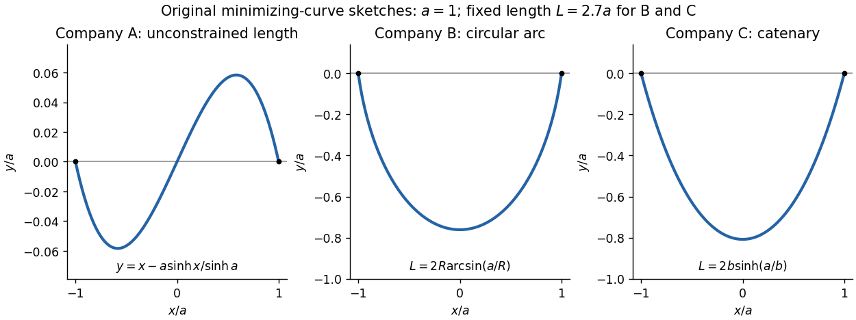
The endpoint constraints are $y(-a)=y(a)=0$. The constants in the three costs contribute only $2aK$, $2a{K}^{\prime }$ and $2a{K}^{\prime \prime }$ respectively, so they do not affect the minimizing shapes. For companies B and C, the fixed arc length isThe original PDF has $(y^{\prime }{)}^2$ as company A's first variable term. The local TeX transcription has lost that derivative dot and incorrectly repeats $y^2$; the calculation below follows the PDF.

Company A. The relevant functional is $J_A=\int (y^{\prime 2}+y^2-2xy)dx$. The Euler-Lagrange equation givesIts general solution is $y=x+c_1\cosh x+c_2\sinh x$. Adding and subtracting the endpoint equations gives $c_1=0$ and $c_2=-a/\sinh a$. ThusThis curve is odd, negative on the left half and positive on the right half; company A has no lower-half-plane restriction. It is the unique global minimum. Indeed, for any endpoint-zero variation $\eta$, integration by parts and the differential equation cancel all linear terms, leavingunless $\eta =0$.

Company B. Minimize $\int ydx$ under the length constraint. Introduce a constant Lagrange multiplier $\lambda$ and apply the Euler-Lagrange equation to $y+\lambda \sqrt{1+y^{\prime 2}}$:The curvature is constant, so the required lower arc is a circular arc. Writing its radius as $R\ge a$ and imposing the endpoints givesSince $\sqrt{1+y_B^{\prime 2}}=R/\sqrt{R^2-x^2}$, its length determines the radius:Equivalently, introduce $0<\theta \le \pi /2$ with $a=R\sin \theta$. Then $L/(2a)=\theta /\sin \theta$, which increases strictly from $1$ to $\pi /2$. The stipulated range of $L$ therefore selects one minor arc. At $L=\pi a$ it becomes the lower semicircle, with vertical endpoint tangents; it is still a single-valued finite-length graph.

Global minimality follows from the convexity of the augmented slope cost with $\lambda =R$. For a competitor $y=y_B+\eta$,Consequently the augmented cost difference is at least $\int (\eta +x{\eta }^{\prime })dx=[x\eta {]}_{-a}^a=0$. Competitors have the same length, so the multiplier contribution cancels and the original cost is minimized. This proves that a circular arc maximizes area below a fixed chord: minimizing negative signed height maximizes the area between the fence and the chord.

Company C. The variable cost is $J_C=\int yds=\int y\sqrt{1+y^{\prime 2}}dx$. The augmented integrand is $(y+\lambda )\sqrt{1+y^{\prime 2}}$. Since it has no explicit $x$ dependence, the Beltrami identity givesThe hanging branch with $b>0$ integrates to $y+\lambda =b\cosh [(x-x_0)/b]$. Equal endpoint heights force $x_0=0$, and the endpoint value fixes $\lambda =b\cosh (a/b)$. ThusIts length isWriting $q=a/b$, the equation $L/(2a)=\sinh q/q$ has one positive solution for every $L>2a$: its derivative has numerator $q\cosh q-\sinh q>0$. The curve is a catenary, is even, and lies strictly below the chord except at the endpoints.

A direct argument proves this is a global minimum, rather than merely an extremum of an augmented functional. Parametrize any competitor by arc length $s\in [-L/2,L/2]$, from its left endpoint to its right endpoint. Then $x^{\prime 2}+y^{\prime 2}=1$, $\int x^{\prime }ds=2a$, and integration by parts givesThe Cauchy-Schwarz inequality gives the last step. Equality requires $x^{\prime }=b/\sqrt{b^2+s^2}$ and $y^{\prime }=s/\sqrt{b^2+s^2}$, whose integrals are precisely the displayed catenary with the stated length. Thus it attains a lower bound valid for every competitor. This proves that a catenary minimizes the integral of height along a fixed-length curve.

The sketch uses $a=1$ and $L=2.7$ for the two fixed-length cases. The vertical scale in the company A panel is enlarged to show its small odd deflection. No comparison between the three companies' absolute prices is required or possible from the shapes alone, since their additive cost constants are independent.

Choose homogeneous Dirichlet boundary conditions $\psi (a)=\psi (b)=0$, and take a nonzero real admissible trial $\psi$. Write the numerator as $F[\psi ]$ and denominator as $G[\psi ]>0$. For an endpoint-zero variation $\eta$, integration by parts givesThus the first variation of the Rayleigh quotient isBy the fundamental lemma of the calculus of variations, stationarity is equivalent toConversely, multiplying an eigenfunction equation by $\psi$ and integrating gives $F=\lambda G$, so its first variation vanishes. This establishes the equivalence for the chosen Sturm-Liouville problem. Homogeneous Neumann boundary conditions, or a mixed Dirichlet-Neumann pair, also cancel the boundary term; general Robin boundary conditions require adding the corresponding boundary contribution to the numerator.

The original PDF has a typographical omission: its displayed equation has $\lambda w(x)$ rather than $\lambda w(x)y(x)$ on the right. Taken literally, it is an inhomogeneous boundary value problem, not the stated Sturm-Liouville problem. The quotient and the later eigenfunction expansion identify the intended equation, which the following derivation produces explicitly.

Choose homogeneous Dirichlet boundary conditions $y(a)=y(b)=0$ and a nonzero real admissible $y$. Then $G[y]>0$ because $w>0$. For an endpoint-zero variation $\eta$, integration by parts givesThe first variation of the Rayleigh quotient is thusBy the fundamental lemma of the calculus of variations, stationarity is equivalent toConversely, multiply this corrected eigenvalue equation by $y$ and integrate. The same boundary cancellation gives $F[y]=\lambda G[y]$, so the first variation vanishes. This proves the requested equivalence for the intended equation. Homogeneous Neumann boundary conditions, or a Dirichlet condition at one end and a Neumann condition at the other, also eliminate the boundary term. General Robin boundary conditions would require the corresponding boundary contribution in the numerator.

The Fermat principle states that the actual path of a light ray makes its travel time stationary under small admissible variations with fixed endpoints. Equivalently, its optical path length is stationary:where $v$ is the local light speed, $n$ is the refractive index, and the two integrals differ by the constant vacuum light speed. In a uniform medium this reduces to stationarity of geometric path length. The principle is a stationarity statement; for the planar reflection considered next the stationary path is also the unique minimum.

First expand the variational integrand:Its needed partial derivatives are ${\mathcal{L}}_f=3f^{\prime }+4f$ and ${\mathcal{L}}_{f^{\prime }}=2f^{\prime }+3f-x$. The Euler-Lagrange equation is thereforeThe general solution is $f=A\cosh (\sqrt{2}x)+B\sinh (\sqrt{2}x)-1/4$. Subtracting the two endpoint equations gives $B=0$; adding them gives $A=1/[4\cosh \sqrt{2}]$. HenceThis is the unique stationary solution. It is also the unique global minimizer: after discarding the fixed boundary terms, integration by parts rewrites $I$ as ${\int }_{-1}^1[f^{\prime 2}+2f^2+f-2x^2]dx$. For an endpoint-zero variation $\eta$, the linear part vanishes at the displayed solution andwith equality only for $\eta =0$.

For fixed initial and final coordinates, the two Euler-Lagrange equations areIndeed the first variation of the functional isIntegration by parts moves the time derivatives from the variations; their endpoint values are zero. The fundamental lemma of the calculus of variations then gives the two equations above.

This is an isoperimetric constraint, imposed on the whole path rather than separately at each time. Introduce a constant Lagrange multiplier $\lambda$ and replace the variational integrand by $\tilde{f}=f+\lambda u$. The modified Euler-Lagrange equations areSolve these together with the fixed endpoint conditions, treating $\lambda$ as an unknown constant, then choose its value so thatThe multiplier is constant because there is one scalar integral constraint. A condition imposed at every time would instead call for a time-dependent multiplier. As usual, this multiplier procedure assumes the constraint is regular, so its first variation does not vanish identically on all admissible variations.

Impose $y=x$ before varying. Writing $\delta ={\delta }_1+{\delta }_2$, the restricted integrand isIts middle term is the total derivative of $\alpha ({\gamma }_1+{\gamma }_2)(x+\beta x^2/2)$, so it can be dropped for fixed endpoints by part (b). The remaining Euler-Lagrange equation is $\delta \ddot{x}=\alpha \beta$. Integrating twice and imposing $x(0)=0$, $x(T)=S$ givesThis is the unique global minimizer among paths on the specified line. To prove it, add any admissible variation $\eta$ with $\eta (0)=\eta (T)=0$. The change in fuel, after dropping the fixed boundary term, isThe first integral vanishes by integration by parts and the equation for $x$. Equality forces $\eta =0$. No monotonicity or restriction to the segment between endpoints was imposed in the question; the minimizing coordinate can initially decrease for sufficiently large $T$.

Take nonzero real trial functions $y$ with $y,y^{\prime }$ square-integrable and sufficient decay for integration by parts. For a compactly supported variation $y\mapsto y+\epsilon \eta$, the first variations areThe quotient rule for the functional then yieldsBy the fundamental lemma of the calculus of variations, stationarity for all such $\eta$ is equivalent toConversely, multiplying a decaying eigenfunction equation by $y$ and using integration by parts gives $F[y]=EG[y]$, so its Rayleigh quotient equals $E$ and its first variation vanishes. Thus the stationary values of the functional are the energy eigenvalues. The word "extrema" in the question includes stationary points here: higher eigenfunctions can be saddle points of the unrestricted Rayleigh quotient.

The Rayleigh-Ritz variational principle givesChoose an admissible trial family, calculate its Rayleigh quotient, and minimize over its parameters to obtain the best upper bound within that family. Equality holds for the exact ground state; a restricted family generally gives only an upper bound.

Let $\eta$ be a smooth variation with $\eta (a)=\eta (b)=0$. Assuming the usual continuous second derivatives of $F$, stationarity of the functional under $y+t\eta$ gives its first variationIntegration by parts removes the derivative of $\eta$; its boundary term vanishes because the endpoint values are fixed. Thusfor every such variation. The fundamental lemma of the calculus of variations implies the Euler-Lagrange equation $F_y=(d/dx)F_{y^{\prime }}$.

For arc length, $F=\sqrt{1+(y^{\prime }{)}^2}$, soThe function $s\mapsto s/\sqrt{1+s^2}$ is strictly increasing; hence $y^{\prime }$ is constant. With endpoints $(a,A)$ and $(b,B)$, $a<b$, the extremal isIt is also the global shortest curve: integrating the unit displacement vector dotted with the curve velocity gives the endpoint distance, which is at most the integrated speed by Cauchy-Schwarz inequality; the straight segment attains equality. A vertical segment is described parametrically or after rotating axes, since it cannot be represented by $y(x)$ on a nontrivial horizontal interval.

Take a smooth variation $u+\epsilon \eta$ with $\eta$ vanishing on the boundary; compactly supported test functions suffice for the interior equation. At an extremum, the first variation is zero:Integration by parts removes the derivatives from $\eta$. The boundary terms vanish, givingThe fundamental lemma of the calculus of variations gives the Euler-Lagrange equationThis is the classical equation for sufficiently smooth admissible extrema; for weaker regularity the first-variation identity supplies its weak form.

For the squared-gradient integrand, the equation is $2(u_{xx}+u_{yy}+u_{zz})=0$, namely the Laplace equation. Put $u_0=ax+by+cz$ and write any admissible function as $u=u_0+v$, with $v=0$ on the boundary. The energy identity isBy the divergence theorem, the middle integral is ${\int }_{\partial V}v(a,b,c)\cdot ndS=0$; equivalently it vanishes by weak integration by parts for zero-trace functions. The final term is nonnegative and vanishes at $v=0$. Thus this is a global minimum, not merely a stationary value:

Let $P=F_{y^{\prime }}$ and $Q=F_{y^{\prime \prime }}$. For a smooth variation $y+\epsilon \eta$, the first variation isHere the last expression follows by two integrations by parts. Taking variations supported in the interior and applying the fundamental lemma of the calculus of variations gives the Euler-Lagrange equation for a second-derivative functional:If both endpoint values and slopes are free, their independent variations force the natural boundary conditions for second-derivative functionalsIf an endpoint value or slope is fixed instead, its corresponding variation vanishes and the associated natural condition is not required.

For $H=y^{\prime \prime }Q-y^{\prime }(Q^{\prime }-P)-F$, differentiate using the chain rule:The Euler-Lagrange equation cancels the first term. Consequently $H^{\prime }=-F_x$, and if there is no explicit $x$ dependence,This is a Beltrami identity for a second-derivative functional.

Take independent smooth variations $y+\epsilon \eta$ and $z+\epsilon \zeta$. Differentiating the functional and using integration by parts gives its first variationFirst choose variations vanishing at the endpoints. To use the stated form of the fundamental lemma of the calculus of variations, take $\eta =(x-a)(b-x)\chi$ with arbitrary smooth $\chi$, and similarly for $\zeta$. The lemma makes $(x-a)(b-x)(F_y-d{F}_{y^{\prime }}/dx)$ vanish, and hence makes the unweighted coefficient vanish in the interior; continuity extends this to the endpoints. Applying the same argument to $z$ gives the Euler-Lagrange equationsIf either endpoint value of $y$ or $z$ is free, the corresponding variation there is arbitrary. The remaining boundary term gives the natural boundary conditions for a free endpoint: $F_{y^{\prime }}=0$ for a free $y$ value and $F_{z^{\prime }}=0$ for a free $z$ value at that endpoint. With both coordinates free at both endpoints, all four conditions apply.

For the specified integrand these equations reduce toand the natural conditions are $y^{\prime }=z^{\prime }=0$ at each free endpoint. Eliminating $z$ givesIts four independent modes give the full general solutionAt zero, $y^{\prime }(0)=C+2D$ and $z^{\prime }(0)=2C+D$. Vanishing forces $C=D=0$, givingAt $x=\pi /6$ the two derivative conditions become $A/2+\sqrt{3}B=0$ and $A+\sqrt{3}B/2=0$. Their coefficient determinant is nonzero, so $A=B=0$. Thus the unique stationary extremal with all four natural boundary conditions is $y=z=0$. The word extremal here means a stationary point of the functional; the indefinite integrand does not require this point to be a minimum.

For a variation $y+\epsilon \eta$ with $\eta (0)=\eta (1)=0$, stationarity givesThe boundary term vanishes. The fundamental lemma of the calculus of variations therefore gives the Euler-Lagrange equation $d{F}_{y^{\prime }}/dx-F_y=0$.

Differentiating the proposed first integral givesThus it is constant along an extremal when $F_x=0$, proving the Beltrami identity.

For the positive branch relevant to the endpoint data, $F=\sqrt{1+y^{\prime 2}}/y$. The identity becomesThe Euler-Lagrange equation itself gives $y{y}^{\prime \prime }=-(1+y^{\prime 2})$, so $(y^2{)}^{\prime \prime }=-2$. Integrating, or solving the first integral, yields a circle $y^2+(x-c{)}^2=R^2$. The equal endpoint values force $c=1/2$ and $R^2=5/4$. Hence the unique positive smooth extremal isIt stays positive on the entire interval and satisfies the second-order equation, including its turning point. Merely differentiating the first integral after dividing by $y^{\prime }$ would need extra care there. Geometrically this is an arc of a hyperbolic geodesic in the upper half-plane model.

For the regular Sturm-Liouville setting assume $p$ is positive and continuously differentiable, $q,w$ are continuous, and $w>0$. Apply a multiplier to $J[y]-\lambda ({\int }_a^{b}w{y}^2-1)$. Its first variation, divided by two, isEndpoint-vanishing variations and the allowed fundamental lemma giveIf an endpoint value is free, its variation is arbitrary, giving the natural condition $p{y}^{\prime }=0$ at that endpoint. At a prescribed endpoint value the variation vanishes there, so no additional natural condition is imposed.

For eigenfunctions $u,v$ with different eigenvalues, multiply their equations by $v,u$ and subtract after integration. The resulting boundary expression $[p(u{v}^{\prime }-u^{\prime }v){]}_a^b$ vanishes under common homogeneous Dirichlet or common natural boundary conditions. Hence $({\lambda }_u-{\lambda }_v){\int }_a^{b}wuv=0$, proving weighted orthogonality.

For the final Dirichlet problem the normalized stationary modes areSolving $y^{\prime \prime }+(\lambda +1)y=0$ with both endpoint values zero gives these and excludes nonpositive $\lambda +1$. Distinct sine modes have zero integral product on $[0,1]$. Their Dirichlet values also make the same boundary expression vanish, which explains orthogonality even though their endpoint derivatives do not obey the natural conditions.

For global minimality, the Fourier sine expansion of an endpoint-vanishing function and Parseval's identities give $\int y^{\prime 2}=\sum k^2{\pi }^2{a}_k^2\ge {\pi }^2\sum a_k^2={\pi }^2\int y^2$. Equality holds exactly in the first sine eigenspace. ThereforeDistinct modes are orthogonal; the two sign choices of the same minimum are not orthogonal to each other. This distinguishes the family of stationary modes from the two representatives of the minimizing eigenspace in the question's wording.

For a normal sample of size $m$,Then $\bar{X}\sim N({\mu }_X,{\sigma }^2/m)$ and $c{S}_X^2\sim {\chi }_{m-1}^2$ with $c=(m-1)/{\sigma }^2$. These two statistics are independent.

Combining the difference distribution and pooled variance calculation gives, with $\nu =m+n-2$,The printed statistic has the sign of the centering term reversed. Its numerator subtracts ${\mu }_Y-{\mu }_X$, so it is not generally a central Student statistic; the corrected centering above is necessary. Under the null hypothesis ${\mu }_X={\mu }_Y$, the two expressions coincide, so the requested test is unaffected. Reject the two-sided null at significance level $\alpha$ whenHere $\nu =8$ and $|T|=2.19<2.31$, so do not reject at the 5% level. This does not establish equality of the population means.

Age matching means that the two observations in a pair share an age effect, while ages vary across pairs. The independent, identically distributed two-sample model no longer represents this design: random pair effects induce within-pair dependence, and fixed differing ages can instead produce different individual means. Pairing by itself need not cause stochastic dependence when ages are treated as fixed. The appropriate alternative is a paired t-test on the within-pair differences. Removing shared age variation can reduce the noise and improve power when age strongly affects volume and the members of a pair are positively associated. Improvement is not automatic, since the paired test also uses fewer degrees of freedom.

For the regular Sturm-Liouville setting assume $p$ is positive and continuously differentiable, $q,w$ are continuous, and $w>0$. Apply a multiplier to $J[y]-\lambda ({\int }_a^{b}w{y}^2-1)$. Its first variation, divided by two, isEndpoint-vanishing variations and the allowed fundamental lemma giveIf an endpoint value is free, its variation is arbitrary, giving the natural condition $p{y}^{\prime }=0$ at that endpoint. At a prescribed endpoint value the variation vanishes there, so no additional natural condition is imposed.

For eigenfunctions $u,v$ with different eigenvalues, multiply their equations by $v,u$ and subtract after integration. The resulting boundary expression $[p(u{v}^{\prime }-u^{\prime }v){]}_a^b$ vanishes under common homogeneous Dirichlet or common natural boundary conditions. Hence $({\lambda }_u-{\lambda }_v){\int }_a^{b}wuv=0$, proving weighted orthogonality.

For the final Dirichlet problem the normalized stationary modes areSolving $y^{\prime \prime }+(\lambda +1)y=0$ with both endpoint values zero gives these and excludes nonpositive $\lambda +1$. Distinct sine modes have zero integral product on $[0,1]$. Their Dirichlet values also make the same boundary expression vanish, which explains orthogonality even though their endpoint derivatives do not obey the natural conditions.

For global minimality, the Fourier sine expansion of an endpoint-vanishing function and Parseval's identities give $\int y^{\prime 2}=\sum k^2{\pi }^2{a}_k^2\ge {\pi }^2\sum a_k^2={\pi }^2\int y^2$. Equality holds exactly in the first sine eigenspace. ThereforeDistinct modes are orthogonal; the two sign choices of the same minimum are not orthogonal to each other. This distinguishes the family of stationary modes from the two representatives of the minimizing eigenspace in the question's wording.

For a normal sample of size $m$,Then $\bar{X}\sim N({\mu }_X,{\sigma }^2/m)$ and $c{S}_X^2\sim {\chi }_{m-1}^2$ with $c=(m-1)/{\sigma }^2$. These two statistics are independent.

Combining the difference distribution and pooled variance calculation gives, with $\nu =m+n-2$,The printed statistic has the sign of the centering term reversed. Its numerator subtracts ${\mu }_Y-{\mu }_X$, so it is not generally a central Student statistic; the corrected centering above is necessary. Under the null hypothesis ${\mu }_X={\mu }_Y$, the two expressions coincide, so the requested test is unaffected. Reject the two-sided null at significance level $\alpha$ whenHere $\nu =8$ and $|T|=2.19<2.31$, so do not reject at the 5% level. This does not establish equality of the population means.

Age matching means that the two observations in a pair share an age effect, while ages vary across pairs. The independent, identically distributed two-sample model no longer represents this design: random pair effects induce within-pair dependence, and fixed differing ages can instead produce different individual means. Pairing by itself need not cause stochastic dependence when ages are treated as fixed. The appropriate alternative is a paired t-test on the within-pair differences. Removing shared age variation can reduce the noise and improve power when age strongly affects volume and the members of a pair are positively associated. Improvement is not automatic, since the paired test also uses fewer degrees of freedom.

Let $\eta$ be a smooth variation with $\eta ={\eta }^{\prime }=0$ at both endpoints, and consider $y_{ϵ}=y+ϵ\eta$. stationary point gives the first variationIntegrate the middle term once by parts and the last term twice. All boundary terms vanish because both $\eta$ and ${\eta }^{\prime }$ vanish there. Assuming the derivatives needed for the classical formula, the given fundamental lemma of the calculus of variations yieldsWithout assuming those classical derivatives initially, the same calculation with compactly supported variations states this equation weakly; sufficient regularity then gives the classical equation.

For the specific integrand, $F_y=-2y$, $F_{y^{\prime }}=0$, $F_{y^{\prime \prime }}=2y^{\prime \prime }$, so the equation is $y^{(4)}-y=0$. Its weak solutions here are smooth, and its general classical solution isPut $\ell =\pi /2$, $c=\cosh \ell$, $s=\sinh \ell$. The conditions at zero give $C=-A$ and $D=1-B$. Those at $\ell$ giveUsing $c^2-s^2=1$, solve to obtain $A=c/2$, $B=(1-s)/2$, $C=-c/2$, $D=(1+s)/2$. Thus an extremal isSubstitution checks all four boundary values. The additive term $x^2$ in the integrand contributes no variation in $y$, so it does not alter this equation.