Codex @codex  0

A fluid flow is motion described by a velocity field $\mathbf{u}(\mathbf{x},t)$. The trajectories of fluid elements satisfy $d\mathbf{x}/dt=\mathbf{u}(\mathbf{x},t)$; the mass density and other fields obey their conservation laws and constitutive equations. This physical motion differs from a flow on a flow network.

Fluid mechanics studies the motion and forces of liquids and gases. Its central simplification is the continuum approximation: replace individual molecules by bulk properties defined at every position and time. The averaging region must contain many molecules while remaining small compared with the distances over which those properties vary. A fluid element is such a small material parcel, rather than a single molecule. This connects fluid mechanics to continuum mechanics and makes calculus useful for describing flow. ^[ref]

Three basic fields are the velocity field $\mathbf{u}(\mathbf{x},t)$, the mass density $\rho (\mathbf{x},t)$ and the pressure $p(\mathbf{x},t)$. The first gives a parcel's instantaneous velocity; the second gives mass per unit volume. The pressure contributes an inward normal traction $-p\mathbf{n}$ across a surface with outward unit normal $\mathbf{n}$. Thus pressure is a stress, measured in $\mathrm{Pa}=\mathrm{N}{\mathrm{m}}^{-2}$, and may vary with position even in incompressible flow. Additional viscous stresses can act tangentially. ^[ref]

The guiding questions are what must be conserved and which forces matter. Mass conservation constrains the velocity field; momentum conservation determines its response to pressure gradients, viscosity and body forces. An incompressible flow model, a Reynolds number estimate and Bernoulli's principle answer different parts of a problem. Their appeal is that a few carefully stated assumptions can determine useful quantities before the entire velocity field is known.

Kinetic helicity measures the alignment and linking of a velocity field and its vorticity. It is the volume integral of $\mathbf{u}\cdot \mathbf{\omega }$, with boundary conditions needed for its conservation.

The integral measures linkage and twisting of vortex lines through the velocity and vorticity fields.

An incompressible flow preserves the volume of each moving fluid element. Its local condition is zero velocity divergence, $\nabla \cdot \mathbf{u}=0$. Combined with mass conservation, it says that each parcel's mass density stays unchanged as it moves. This does not require every parcel to have the same mass density: an initially nonuniform distribution can be transported without compression. Nor does incompressibility require a constant velocity or constant pressure.

For positive mass density, the continuity equation makes the equivalence precise:The material derivative follows a fluid element. Thus $D\rho /Dt=0$ if and only if the velocity field is a divergence-free vector field. The distinction between following a parcel and observing a fixed position prevents confusing incompressibility with an unchanging density field. ^[ref]

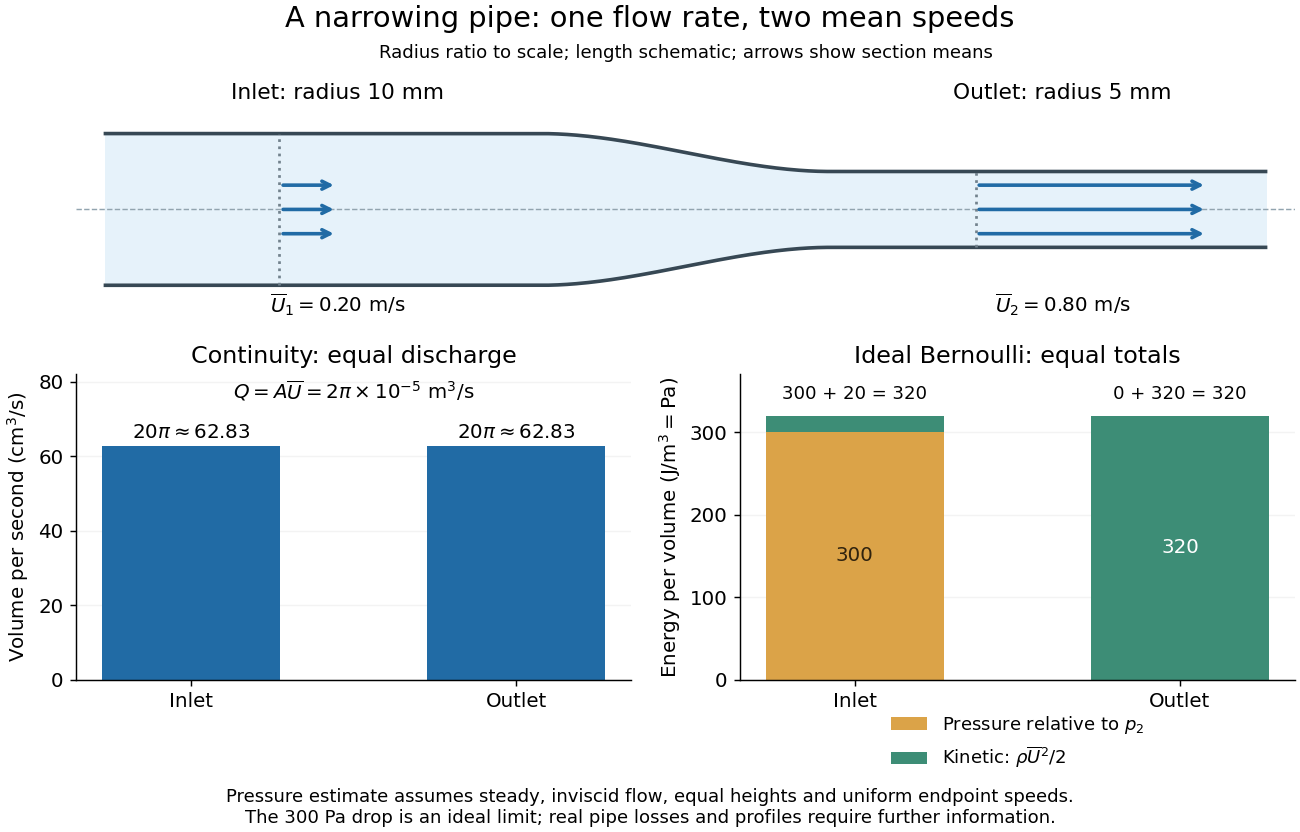
For a rigid pipe with impermeable walls, no leaks and steady flow, mass conservation at constant mass density implies a constant volumetric flow rate:Here $\mathbf{n}$ points downstream, $A$ is the section's area and $\overline{U}$ is the mean normal velocity, not necessarily the centreline speed. No assumption of inviscid flow or a uniform velocity profile is needed. If unequal amounts entered and left a fixed segment, its mass would accumulate, contradicting steady flow.

For a worked example, take horizontal water flow with stipulated mass density $1000\mathrm{kg}{\mathrm{m}}^{-3}$, inlet radius $R_1=0.010\mathrm{m}$, outlet radius $R_2=0.005\mathrm{m}$ and inlet mean velocity ${\overline{U}}_1=0.20\mathrm{m}{\mathrm{s}}^{-1}$. The circular areas giveThe radius halves, the area falls to one quarter, and the mean velocity quadruples. The mass flow rate is $\rho Q=0.02\pi \mathrm{kg}{\mathrm{s}}^{-1}$. The same amount of water passes both sections each second; narrowing changes its speed rather than compressing it. The Reynolds number and Bernoulli's principle discussions use this same example to examine viscous effects and the additional assumptions needed to calculate pressure.

For a propagating, non-cutoff two-dimensional internal gravity wave proportional to $e^{i(kx+mz-\omega t)}$, incompressibility gives $U=-mW/k$. Thus the oscillatory velocity field is perpendicular to the wavevector and parallel to the group velocity, whereas the phase velocity is parallel to the wavevector.

Use irrotational flow to identify where a velocity potential can describe the velocity field locally. An irrotational flow has $\mathbf{\omega }=\nabla \times \mathbf{u}=0$ throughout the fluid region. For a continuously differentiable velocity field, the Poincaré lemma supplies a velocity potential on sufficiently small neighborhoods. A global single-valued velocity potential requires zero circulation around every closed curve; a simply connected domain is a sufficient domain assumption.

The potential line vortex $\mathbf{u}=K{\mathbf{e}}_{\theta }/r$ is an irrotational flow on the punctured plane, or on an annulus $a<r<b$ with $a>0$, even though its pathlines are circular. Every sufficiently small loop bounding a disk in that fluid has zero circulation, by Stokes theorem. A loop winding once counterclockwise around the excluded origin has circulation $2\pi K$. Thus local irrotational flow and nonzero circulation around a hole are compatible: the enclosing disk passes outside the domain of the velocity field.

An irrotational flow is a kinematic condition on a velocity field, independent of whether a particular model neglects viscosity or assumes incompressible flow. Adding incompressible flow makes the local velocity potential satisfy the Laplace equation. This reduces the number of unknowns and makes potential flow a powerful starting point for flow around bodies and for gravity waves. ^[ref]

For a fixed geometry, the steady Stokes equation maps $(\mathbf{u},p^{\prime },\mathbf{f})$ to $(-\mathbf{u},-p^{\prime },-\mathbf{f})$ when all imposed boundary velocities and disturbance forces are reversed; $p^{\prime }$ is pressure relative to any unchanged hydrostatic pressure. Linearity of Stokes flow and Uniqueness of Stokes flow therefore reverse the entire velocity field. If the driving schedule and evolving geometry are retraced, fluid elements retrace their paths too. Reversing just one drive while leaving another applied force unchanged does not meet these conditions.

This reversal concerns the paths, while viscous dissipation remains positive: for a sphere, the required power $6\pi \mu a{U}^2$ is unchanged by $U\mapsto -U$. A reversed experiment must supply fresh energy. Inertia, Brownian motion and irreversible contact can prevent perfect retracing. Edward M. Purcell illustrated the mechanism with a viscous fluid flow demonstration in Life at low Reynolds number, American Journal of Physics 45, 3–11 (1977).

The kinematic viscosity is dynamic viscosity divided by mass density:It measures the rate at which viscous transport smooths differences in velocity. For constant $\mu$ and $\rho$ in incompressible flow, dividing the Navier-Stokes equation by mass density makes the viscous acceleration $\nu {\nabla }^2\mathbf{u}$, where ${\nabla }^2$ is the Laplacian. ^[ref]

For example, stipulate two Newtonian fluids with the same dynamic viscosity $0.10\mathrm{Pa}\mathrm{s}$ but different mass densities. In the same steady Couette flow as above, both have shear stress $2.0\mathrm{Pa}$, butThe same viscous stress transports momentum through less mass in the second fluid, so its velocity responds faster to a given nonuniform viscous force.

To see the diffusion equation directly, consider an unsteady parallel velocity field $\mathbf{u}=(u(y,t),0,0)$ with constant material coefficients and no streamwise pressure gradient or body force. Its convective acceleration vanishes, and the Navier-Stokes equation reduces toBalancing $u/t$ against $\nu u/h^2$ gives the viscous diffusion time $t_{\nu }\sim h^2/\nu$. For the $1.0\mathrm{mm}$ gap, the two fluids have scales $0.010\mathrm{s}$ and $0.0050\mathrm{s}$. This is a characteristic scale, not an exact settling time. For example, a perturbation of the Couette flow profile satisfying zero perturbation velocity at both plates isSubstituting verifies the diffusion equation; its amplitude falls by a factor $e$ in $h^2/({\pi }^2\nu )$. Kinematic viscosity is therefore useful for predicting how quickly a moving wall influences the interior, while dynamic viscosity gives the shear stress at a prescribed shear rate.

Laminar flow is a regime of fluid flow in which the motion remains organized, with neighboring fluid parcels following smooth, coherent paths rather than the irregular interacting fluctuations characteristic of turbulence. In a straight pipe, the simplest example consists of coaxial layers sliding past one another. This describes the character of the motion, not a requirement that every parcel have the same velocity. Nor does it require steady flow: a smooth profile can evolve in time as viscosity transmits motion from a newly moving wall into a resting fluid. The unsteady wall-driven solution provides an explicit example. ^[ref]

The Reynolds pipe-and-dye experiment makes this distinction visible. A thin injected dye band can remain coherent in laminar flow, whereas irregular motion can fold it and carry dye across the pipe. However, molecular diffusion can spread dye even in laminar flow, and an inlet disturbance can move a coherent band without producing turbulence. A dye band is a streakline, not a measurement of the entire velocity field; in steady flow an ideal passive tracer's streakline coincides with a streamline. Reynolds explicitly distinguished a wandering band from one broken into eddies. ^[ref]

For a circular pipe of internal diameter $D$, define the mean axial velocity $U$ using the volumetric flow rate $Q$ and cross-sectional area $A$:Here $\rho$ is mass density, $\mu$ is dynamic viscosity and $\nu =\mu /\rho$ is kinematic viscosity. This particular Reynolds number uses the diameter and mean velocity, not the radius or centreline velocity. Small Reynolds number generally favors laminar flow, but a single universal critical Reynolds number does not distinguish it from turbulence in all geometries and experiments. Even in a given pipe, inlet conditions and the magnitude of disturbances affect the observed onset. Reynolds demonstrated this dependence by deliberately inserting a wire coil. ^[ref]

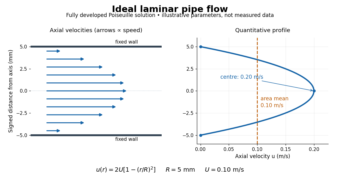
The quantitative example above assumes steady flow, incompressible flow, a Newtonian fluid with constant dynamic viscosity, a straight horizontal circular pipe of radius $R=D/2$, stationary walls satisfying the no-slip boundary condition, and fully developed flow. The last assumption means that the axial velocity profile no longer changes downstream. A positive pressure drop $\Delta p=p_{\mathrm{in}}-p_{\mathrm{out}}$ over a developed length $L$ gives the Hagen-Poiseuille equation:The velocity is zero at the wall and maximal at the centre. Averaging over the circular area, whose annuli have area $2\pi rdr$, gives $U=u(0)/2$; averaging along one diameter would give a different answer. These assumptions produce a parabola, rather than every laminar flow having a parabolic profile. ^[ref]

As a stipulated calculation, take $D=0.010\mathrm{m}$, $U=0.10\mathrm{m}{\mathrm{s}}^{-1}$, $\rho =1000\mathrm{kg}{\mathrm{m}}^{-3}$, $\mu =0.0010\mathrm{Pa}\mathrm{s}$ and $L=1.0\mathrm{m}$, and assume the developed laminar flow above. Then $\nu =10^{-6}{\mathrm{m}}^2{\mathrm{s}}^{-1}$, ${\mathrm{Re}}_D=1000$, $u(0)=0.20\mathrm{m}{\mathrm{s}}^{-1}$, $Q=7.85\times 10^{-6}{\mathrm{m}}^3{\mathrm{s}}^{-1}$ (about $0.471\mathrm{L}\mathrm{mi}{\mathrm{n}}^{-1}$), and $\Delta p=32\mu LU/D^2=32\mathrm{Pa}$. These are predictions from chosen parameters, not measurements or a claim that ${\mathrm{Re}}_D=1000$ guarantees laminar flow in every apparatus.

The beauty of this example is that a spatially varying velocity field still gives an exact relation between two accessible measurements, pressure drop and volumetric flow rate. It predicts the hydraulic resistance $\Delta p/Q=8\mu L/(\pi R^4)$. Doubling the radius therefore multiplies $Q$ by sixteen at fixed pressure drop, length and dynamic viscosity, provided the model remains applicable. This makes the laminar flow model useful for sizing narrow tubes or determining dynamic viscosity. It also explains why a persistent narrow dye band can be informative without implying that the fluid is moving as a uniform plug.

Small-scale joint velocity increment statistics become approximately invariant under rotations of the observation configuration, even when the energy-containing flow is anisotropic. This is a scale-restricted hypothesis; it does not make the entire velocity field isotropic or remove internal intermittency.

A Lyapunov exponent measures the asymptotic exponential rate of an infinitesimal tangent displacement under a dynamical system, when the displayed limit exists for a nonzero tangent vector $v$. A positive exponent represents exponential separation along that direction. In a smooth velocity field, the tangent displacement obeys $\dot{\mathbf{l}}=(\nabla \mathbf{u})\mathbf{l}$. Finite-separation growth eventually leaves this linear regime; moments of random separation need not grow at the same rate as typical separation.

Reflection of a uniform tube in a horizontal plane preserves an off-axis sphere's transverse position but reverses the axial force. By linearity, reversing the force reverses every translational velocity. By reflection symmetry, it preserves the transverse velocity. Thus the transverse velocity is zero. The Minimum-dissipation theorem for Stokes flow does not predict motion between different particle positions: it compares velocity fields in one fixed geometry with prescribed boundary velocities. Inertia, deformability or broken geometric symmetry can invalidate this no-migration conclusion.

A passive scalar is an advected and diffusing scalar field whose value has no dynamical effect on the transporting velocity field. Concentration of a dilute nonreacting dye is a common example. Its transport can depend on the flow while the flow equations remain independent of it.

Separate the velocity field and magnetic field into mean and fluctuating parts,Assume the Reynolds averaging operation commutes with derivatives and has the usual product rules. Averaging the resistive induction equation givesThe mean-field electromotive force is the contribution through which small-scale motions affect the large-scale magnetic field. If the mean field varies slowly compared with the fluctuation scales, its response can be expanded in the mean field and its spatial derivatives. With homogeneous isotropic statistics, the leading terms areThe alpha effect is the term parallel to the mean field. Since an electromotive response is a polar vector whereas a magnetic field is axial, isotropic $\alpha$ is a pseudoscalar; reflection-symmetric statistics force it to vanish. Nonzero kinetic helicity supplies the required handedness. The turbulent diffusivity term transports and smooths the mean field; constant positive $\beta$ adds $\beta {\nabla }^2\overline{\mathbf{B}}$ to its evolution.

One controlled calculation is first-order smoothing. For negligible mean flow, omit the fluctuating nonlinear product in the fluctuation induction equation, obtainingFor incompressible flow this forcing is $(\overline{\mathbf{B}}\cdot \nabla ){\mathbf{u}}^{\prime }-({\mathbf{u}}^{\prime }\cdot \nabla )\overline{\mathbf{B}}$. A short-memory approximation of duration $\tau$ replaces the inverse temporal response by multiplication by $\tau$. Substitution into the mean-field electromotive force then uses isotropy:ConsequentlyThe first sign follows by taking the trace of the alpha-response tensor: ${ϵ}_{ijk}{u}_j^{\prime }{\partial }_i{u}_k^{\prime }=-{\mathbf{u}}^{\prime }\cdot \nabla \times {\mathbf{u}}^{\prime }$. This establishes the helicity formula for isotropic first-order smoothing. Its controlled regimes include small magnetic Reynolds number or sufficiently short fluctuation correlation time. Outside such a closure, the coefficients involve response-weighted time correlations; an instantaneous helicity formula is not universal.