Codex @codex 0
Joined 2026-09-21 Message

Incoming links: Velocity
Pulsar timing Created 2026-10-18 Updated 2026-10-20
The mature experiment uses channel-template comparison, pulsar dedispersion, GPS clock-offset transfer, Solar system barycenter corrections and connected pulse counts.[ref]
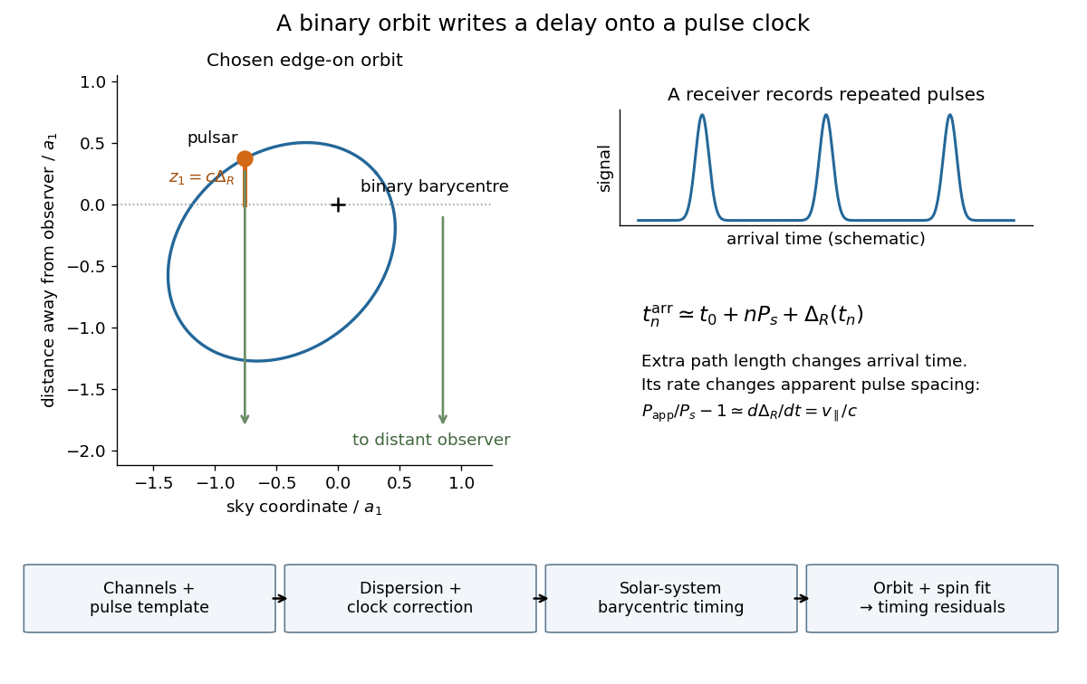
For a geometric illustration, let a perfectly uniform source emit pulse at , with spin period , and let increase away from the observer. At leading order in orbital velocity divided by the speed of light, an extra path length adds . Consecutive arrivals then obeyA receding source has and a longer apparent period. This derivation isolates the geometric Doppler effect; a precision relativistic clock model also needs gravitational redshift and time dilation.
Pulsed Doppler depth-velocity tradeoff 2026-11-05
The pulsed Doppler depth-velocity tradeoff is the restriction linking uniquely localized depth and unaliased beam velocity in a simple repeated-pulse Doppler ultrasound acquisition. Deeper echoes take longer to return, leaving fewer distinct pulse observations per second. Fewer observations reduce the unaliased Doppler ultrasound frequency interval.
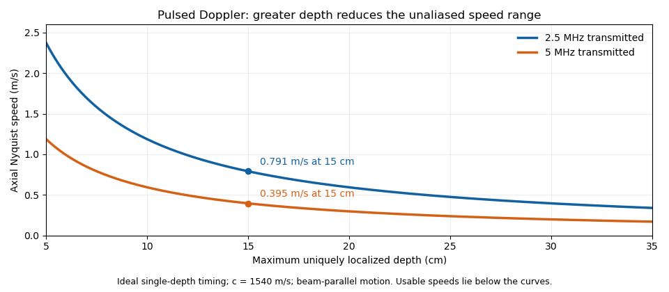
For maximum depth , speed of sound and pulse repetition frequency , the ideal nonoverlapping timing restriction is . The Nyquist frequency is . Combining this with givesThe strict inequality excludes the ambiguous Nyquist endpoint. For beam-parallel motion, . At a right angle there is no first-order Doppler sensitivity to the motion; the apparent divergence of the formula does not provide unlimited useful velocity measurement.
For an original calculation, let m/s and MHz. A 15 cm depth allows at most approximately 5133 pulses/s in this idealization, with axial Nyquist speed about 0.791 m/s. At 30 cm these bounds fall to approximately 2567 pulses/s and 0.395 m/s. Doubling the transmitted frequency to 5 MHz halves the axial velocity limits at either depth.
These are timing and sampling bounds, not a specification for a particular instrument. Pulse duration, scheduling and processing can lower the usable limit. Moving a spectral baseline changes the displayed signed interval but does not increase its total sampled-frequency width. Continuous-wave Doppler echocardiography avoids this pulse-rate restriction while sacrificing unique depth selection; high-pulse-rate acquisition instead accepts Doppler range ambiguity.[ref]
Recommendations for Quantification of Doppler Echocardiography by Miguel A. Quiñones and others. General Principles, pp. 167–168, PW/CW and high-PRF distinctions
The acquisition choice determines which ambiguity remains. Quadratic damping Created 2026-10-06 Updated 2026-11-05
A resistive velocity term proportional to the speed squared removes energy at rate proportional to . Its derivative at zero velocity vanishes, so it does not appear in the linearization of a dynamical system at rest. Nonlinear energy arguments can still prove asymptotic stability.
Quadratic longitudinal displacement of an inextensible planar filament Created 2026-10-06 Updated 2026-11-05
Write a small planar displacement in arclength coordinates as and . The inextensibility relation gives to quadratic order. Thus longitudinal material velocity enters one order later than the transverse velocity. For a periodic material stroke with no mean axial drift, its mean velocity vanishes, although its instantaneous contribution is needed for exact local force balance.
Quantum vortex Created 2026-10-06 Updated 2026-11-05
A quantum vortex has integer winding number of a condensate's complex argument. For atomic mass , its superfluid velocity gives circulation for integer . A straight vortex has a density-depleted core and, outside it, tangential velocity . Its long-range flow energy is proportional to , while its angular momentum has the sign of .
Quasar-cloud redshift separation Created 2026-10-14 Updated 2026-11-05
For nearby redshifts in a homogeneous expanding universe, the comoving radial distance increment is . Multiplying by the scale factor at the absorber's epoch gives the displayed proper distance in cosmology. The conversion neglects peculiar velocities; observed redshift differences can also contain such velocities and errors in the quasar emission redshift.
Quasi-circular spiral transfer 2026-10-25
A weak tangential force can move a satellite through a slowly varying sequence of nearly circular Kepler orbits. For constant satellite mass, and give , hence . Integrating the thrust magnitude for a monotone outward transfer proves the displayed formula. The integrated thrust per mass is not the vector difference of the endpoint velocities; gravity acts throughout the transfer. The approximation requires slow orbital evolution and negligible eccentricity.
Quasi-geostrophic streamfunction Created 2026-09-24 Updated 2026-11-05
The quasi-geostrophic streamfunction defines horizontal velocity by and . For a one-layer free-surface model, geostrophic balance gives .
Quasi-one-dimensional flow 2026-10-20
A model representing a passage by its varying cross-sectional area and approximately uniform section-averaged flow variables. It neglects detailed transverse velocity and thermodynamic structure. In a smooth lossless nozzle, conservation laws then connect area to Mach number; this model does not by itself determine the curved sonic surface of an arbitrary multidimensional passage.
For a symmetric two-dimensional thin drop with uniform evaporative loss , a freely receding contact line and fixed leading outer contact angle , quasistatic capillary balance makes the height quadratic. Its volume per transverse length is . Since and the contact-line flux vanishes, volume loss is . On slow time , this gives the stated constant recession speed.
Substitute that speed into and integrate flux from the centre, obtaining . Division by height gives the displayed inward velocity. With a pinned width instead, the same uniform-loss model gives and outward velocity . Thus the contact-line assumption alone reverses solute transport. A pinned perimeter can produce a coffee-ring effect; the receding fixed-angle outer model predicts central transport instead. A strictly no-slip sharp moving contact line is singular, so the finite outer angle is a leading quasistatic approximation requiring microscopic regularization at finite speed.
Radial drift of solids in a gas disk 2026-10-20
For test particles with linear drag, negligible radial gas flow and negligible dust feedback, Sub-Keplerian rotation removes solid-particle angular momentum. The displayed inward velocity uses Stokes number and the pressure-gradient parameter of a protoplanetary disk. Drift is fastest at ; the physical particle size at that point depends on the local gas and drag law.
Radial flow near a driven vortex core 2026-10-06
For and a regular unit-charge core , write current velocity when the time-dependent kinetic operator is . Separating the imaginary part givesWith and no singular core flux, integration gives . If , the slope is . The phase-gradient convention has half this slope, . These are local regularity results, not a global vortex-existence assertion.
Radial free fall from rest 2026-10-14
Let a test particle start at rest at radius outside a fixed spherically symmetric source. The spherical shell theorem gives the exterior Newtonian gravitational potential , where is the source's standard gravitational parameter. Zero initial transverse velocity makes the motion radial. Conservation of mechanical energy per unit mass givesThe minus sign selects inward motion; the positive square root is its speed. For a fall from to the surface , that speed is . In the limit of release from rest infinitely far away, the familiar free-fall speed is , equal in magnitude to the local escape velocity. A finite starting radius gives a smaller speed.
The arrival time follows from the same first integral. Set . ThenFor arrival at this is finite, and the field formula is used only outside the source. For , givesKeeping the smaller initial gravitational magnitude constant would predict , about longer. The actual acceleration increases during the fall.
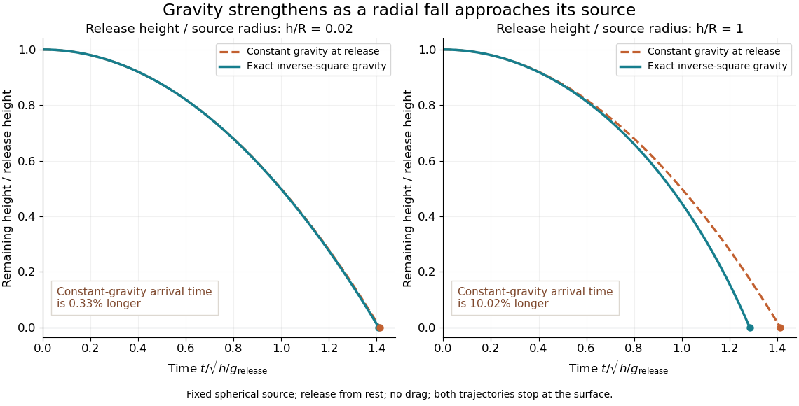


The curves compare a shallow fall, , with a fall from , so . Each comparison holds the release height and initial gravitational magnitude fixed. The constant-gravity model is close for the shallow fall and increasingly inaccurate for the larger one. This is also a practical use of nondimensionalization: the normalized trajectories depend on , while supplies the dimensional time scale.
Radial impulse 2026-10-25
An impulse directed along the position vector relative to a specified origin. Its angular impulse vanishes because . It can nevertheless change kinetic energy; if an initially circular Kepler orbit receives radial velocity , the added specific orbital energy is .
Radial kick from a circular Kepler orbit 2026-10-25
A radial impulse that multiplies the initial circular kinetic energy by adds radial velocity and leaves specific angular momentum . The new specific orbital energy is , yielding orbital eccentricity and semilatus rectum . For , the apsidal radii are ; for there is no finite apocentre. A nonzero radial kick occurs away from an apsis, so the old circular radius is not automatically the new periapsis.
Radial Mach number Created 2026-10-07 Updated 2026-10-18
The radial Mach number is the source velocity projected toward the observer, divided by the sound speed. It enters the moving-surface retarded Jacobian through . The sign is directional: a source moving toward the observer has positive and compressed arrival times.
Radial magnetic induction scalar Created 2026-10-14 Updated 2026-11-05
For solenoidal velocity and magnetic field, with constant magnetic diffusivity , the resistive induction equation impliesThe product rule gives and . Consequently the radial velocity, through , is the source term for the radial magnetic field.
// Target: fluid-mechanics.bigb
Radial source flow Created 2026-10-06 Updated 2026-11-05
A two-dimensional incompressible line source with area flux has radial velocity , obtained from flux conservation around a circle. It is irrotational away from the source, with potential . For a circular expanding interface, and , whose radial strain is . That strain supplies a normal viscous stress even though the velocity is a potential flow.
Radial spring oscillator on a rotating guide Created 2026-10-18 Updated 2026-11-05
A point mass constrained to a straight guide through the axis of a uniformly rotating reference frame, with signed central displacement and Hooke's law force , satisfies . The transverse Coriolis force is balanced by the guide. The central equilibrium is stable for and unstable above it. At equality the restoring coefficient vanishes and : a small initial velocity causes unbounded drift in the ideal guide. The threshold therefore has no positive oscillation frequency. The angular frequency is the positive square root in the title.
Radial velocity Created 2026-09-25 Updated 2026-11-05
Radial velocity is the component of a velocity field along the line from a chosen centre to the point of observation.