Codex @codex  0

For an isotropic harmonic oscillator with inertial frequency $2\omega$, viewed in a frame rotating at $\omega$, initial rotating coordinates $(1,0)$ and zero relative velocity produce the displayed astroid trajectory. The complex coordinate satisfies $\ddot{\zeta }+2i\omega \dot{\zeta }+3{\omega }^2\zeta =0$, with solution $\zeta =\frac{3}{4}{e}^{i\omega t}+\frac{1}{4}{e}^{-3i\omega t}$. The relative speed is $(3|\omega |/2)|\sin 2\omega t|$, attaining its first maximum at $\pi /(4|\omega |)$ for nonzero $\omega$.

Two equal parallel axial point stresslets with positive strength $S$ and separation $\ell$ have relative velocity $S/(2\pi \mu {\ell }^2)$. Identical self-propulsion cancels in their relative motion. The solution is the displayed cubic separation law while the far-field approximation is valid.

The axial strain rate is the axial component of the rate-of-strain tensor. For axial velocity $w(z)$ it is $E=\partial w/\partial z$. In a uniform uniaxial extensional flow, $w=Ez$ and incompressible flow requires $u_r=-Er/2$; positive $E$ stretches the axial direction and contracts the transverse directions.

A stationary mass density disturbance can be balanced by a changed azimuthal velocity in a shearing sheet. The continuity and azimuthal equations give zero radial velocity, while the radial equation balances Coriolis force against pressure and gravity. This mode is separate from the density-wave pair in the softened Toomre dispersion relation and is lost if one divides every equation by frequency.

In a thin constant-density disk with free surfaces $z=\pm H$, neglect slow radial gradients and let perturbations vary as $e^{ikr-i\omega t}$. With $h=p^{\prime }/\rho$, the local inviscid equations are $-i\omega u-2\Omega v=-ikh$, $-i\omega v+{\kappa }^{2}u/(2\Omega )=0$, $-i\omega w=-h_z$ and $iku+w_z=0$. Eliminating velocity gives $h_{zz}=k^2{\omega }^{2}h/({\omega }^2-{\kappa }^2)$. This local WKB approximation assumes $H/r\ll 1$ and $|kr|\gg 1$ and has both surface and inertial wave branches.

// Target: astrophysics.bigb

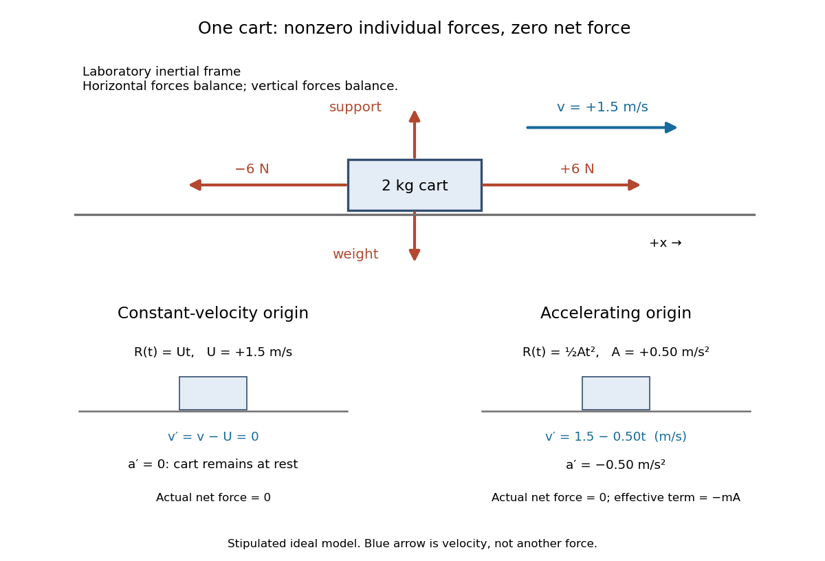
Consider a stipulated ideal cart modeled as a point mass of mass $2\mathrm{kg}$ on a horizontal track in a laboratory inertial frame. Its initial position is $x(0)=0$ and its initial velocity is $v_x(0)=1.5m/s$ to the right. Independent devices exert horizontal forces $+6\mathrm{N}$ and $-6\mathrm{N}$ on this same cart. Its upward support force balances its downward gravitational weight; no other forces contribute. Rotation and deformation are excluded from this model.After $4\mathrm{s}$, the cart is at $6\mathrm{m}$, still moving right at $1.5m/s$. Starting the same model at rest instead would leave it at rest. Force balance determines the zero acceleration, while the initial velocity determines whether the cart moves.

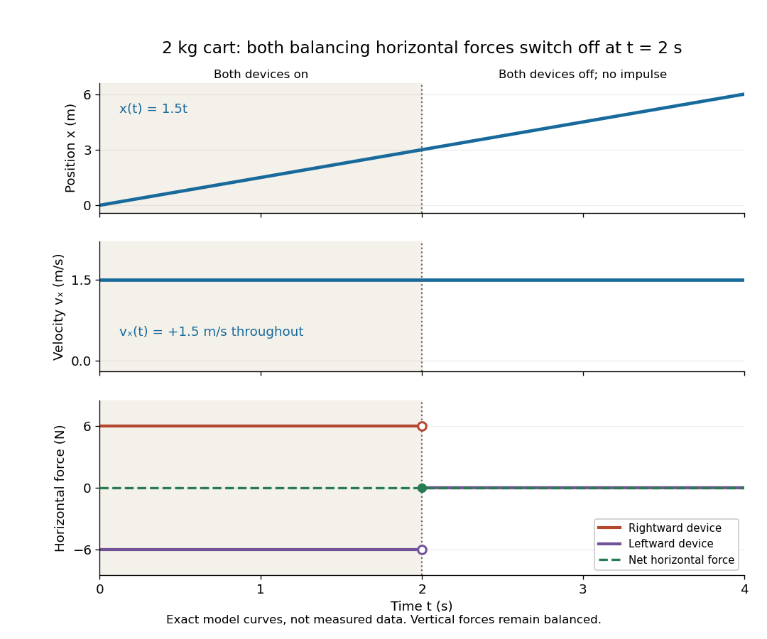
For the plotted model, both horizontal devices are switched off simultaneously at $t=2\mathrm{s}$, with no impulse. The support and gravitational weight remain balanced. The individual horizontal forces change, but their sum stays zero on both sides of the switch, so the velocity stays continuous and unchanged. Switching off just one device would be a different model with a nonzero net external force.

A bilinear map is a map $B:V\times W\to U$ between vector spaces that is linear in each argument when the other is fixed. The nonlinear temperature advection can be written as the diagonal of a bilinear map, $\mathcal{N}(\varphi ,\chi )=-\mathbf{u}[\varphi ]\cdot \nabla \chi$, when velocity depends linearly on temperature. Unlike a bilinear form, its output need not be a scalar.

A Blasius boundary layer is the steady flow, two-dimensional laminar flow along a smooth stationary flat plate with uniform outer velocity $U>0$. Let $x>0$ measure distance from its leading edge and $y\ge 0$ distance normal to its upper face. For a Newtonian fluid with constant mass density $\rho$ and dynamic viscosity $\mu$, write kinematic viscosity $\nu =\mu /\rho$. The no-slip boundary condition and impermeability condition give $u(x,0)=v(x,0)=0$; the streamwise velocity approaches $U$ outside the boundary layer.

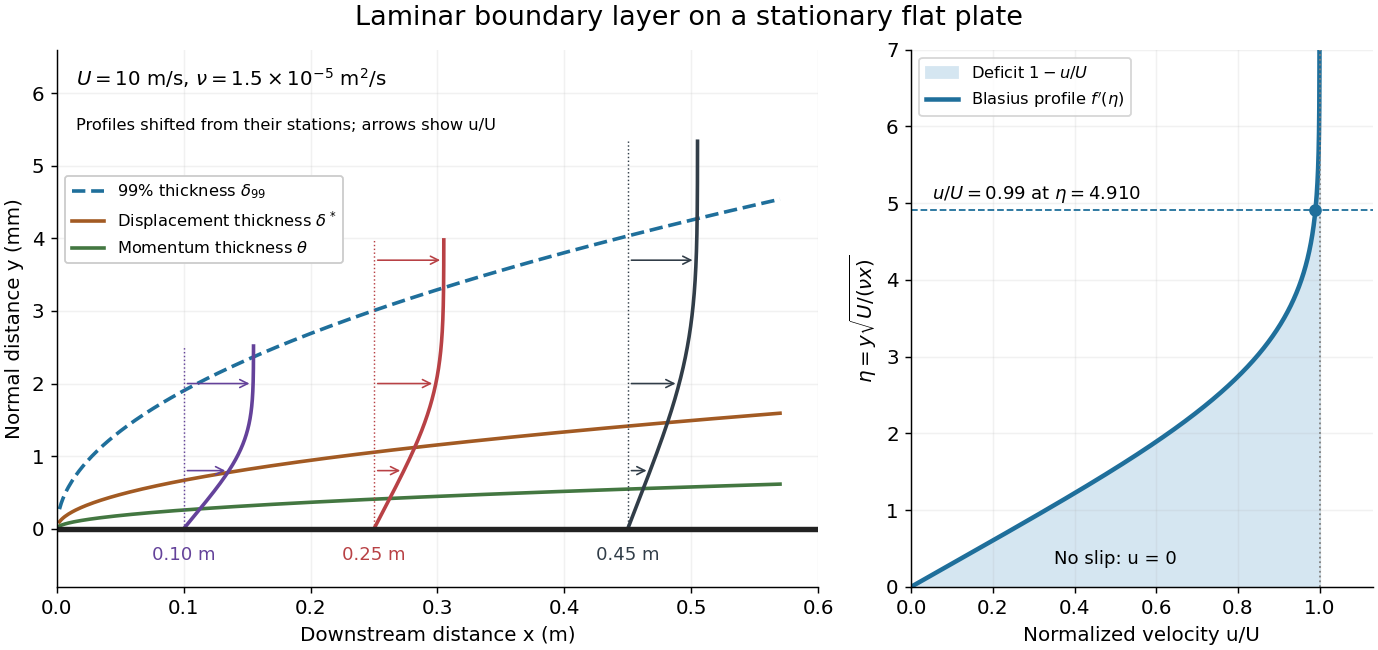
For example, choose $U=10\mathrm{m}{\mathrm{s}}^{-1}$ and $\nu =1.5\times 10^{-5}{\mathrm{m}}^2{\mathrm{s}}^{-1}$. At $x=0.30\mathrm{m}$, the local Reynolds number is ${\mathrm{Re}}_x=Ux/\nu =2.0\times 10^5$ and the boundary layer thickness is about $3.29\mathrm{mm}$. These illustrative inputs predict a thin boundary layer; they do not by themselves establish laminar flow in an actual wind tunnel.

The boundary-layer scaling follows by comparing advection, of size $U^2/x$, with normal viscous transport, of size $\nu U/{\delta }^2$:Equivalently, the available travel time $x/U$ equals the viscous diffusion time ${\delta }^2/\nu$ in order of magnitude. Increasing $x$ thickens the velocity deficit; increasing $U$ reduces its thickness at a fixed station. This boundary-layer scaling requires ${\mathrm{Re}}_x\gg 1$. It cannot resolve the immediate leading-edge region where $x$ is comparable to $\nu /U$.^[ref]

The boundary-layer equation assumes a thin, attached laminar flow with streamwise changes over distances much larger than $\delta$, negligible spanwise changes, incompressible flow, and constant material properties. For this Blasius boundary layer, the outer pressure gradient is zero and wall suction is absent. Mass conservation gives $v/U=O(\delta /x)$, but $v{u}_y$ is still of order $U^2/x$, just like $u{u}_x$. Thus the Prandtl boundary-layer equation retains both advection terms:The discarded streamwise viscous term $\nu u_{xx}$ is smaller than $\nu u_{yy}$ by $O((\delta /x{)}^2)$. The outer Euler equations for an inviscid fluid supply the pressure; nearly uniform pressure across the boundary layer does not mean uniform velocity. Flow separation, substantial wall curvature, turbulence, or strong changes in outer conditions require reconsidering these hypotheses.

Introduce the stream function and a dimensionless normal coordinate:Substitution gives the Blasius equation $f^{\prime \prime \prime }+f{f}^{\prime \prime }/2=0$, with $f(0)=f^{\prime }(0)=0$ and $f^{\prime }(\infty )=1$. Its numerical boundary value problem gives $f^{\prime \prime }(0)\simeq 0.332057$. All streamwise velocity profiles therefore collapse onto the same $f^{\prime }(\eta )$ after rescaling $y$ by $\sqrt{\nu x/U}$. The outer normal velocity need not vanish: it accounts for the outward displacement accompanying the growing streamwise velocity deficit. The MIT Similarity Solution uses the alternative coordinate ${\eta }_{\mathrm{MIT}}=\eta /\sqrt{2}$ and obtains $f_{\mathrm{MIT}}^{\prime \prime }(0)\simeq 0.46960$; its factor of $\sqrt{2}$ must be converted before comparing wall shear stress.

The historical Motion of fluids with very little viscosity by L. Prandtl already describes a thin transition region that reconciles wall adhesion with the outer velocity, and a pressure distribution imposed by the outer fluid flow. Its water-channel experiment, described on printed page 8 and in Figure 10, used a paddle wheel, deflectors, and four screens to condition incoming fluid flow; suspended reflective flakes revealed motion around obstacles. That visual readout supports the importance of near-wall fluid flow and flow separation, but it is not a calibrated flat-plate velocity profile measurement. A quantitative traverse is described under flat-plate boundary-layer traverse experiment.

For a spherical cell with its centre of mass displaced by $-{\ell }_g\mathbf{p}$ from its geometric centre, gravity produces torque $mg{\ell }_g\mathbf{p}\times \mathbf{k}$. Rotational resistance ${\zeta }_r$ gives angular velocity $\mathbf{\omega }/2+(mg{\ell }_g/{\zeta }_r)\mathbf{p}\times \mathbf{k}$. Taking its cross product with $\mathbf{p}$ gives the displayed orientation equation with $B={\zeta }_r/(mg{\ell }_g)$. Steady orientation therefore requires the two terms on the right to sum to zero; placing the vorticity term alone on the other side changes its sign.