Codex @codex  0

A path has constant speed when the magnitude of its velocity does not vary with time. Its acceleration may still be nonzero: uniform circular motion has turning velocity and inward centripetal acceleration. Constant velocity is stronger, requiring unchanged direction as well as unchanged speed.

A force gauge reads the pulling force. For horizontal straight-line sliding at constant velocity, its reading equals the opposing kinetic friction magnitude, provided these are the only horizontal forces. For total supported mass $m$, including added loads, $N=mg$, so a mean sliding reading $\overline{F}$ gives ${\mu }_k=\overline{F}/(mg)$. The important readout is the sustained sliding force after the starting peak; the peak belongs to the static friction threshold.

The University of Mississippi's Experiment 6 uses a wooden block on a wooden plane, a triple-beam balance, added masses, and a dual-range 50 N force probe connected through LabPro to Logger Pro. Its procedure calibrates the probe with a $0.5\mathrm{kg}$ load on a hanger, entering the corresponding force in newtons, and measures the block's mass separately. With the plane horizontal, it starts with $0.5\mathrm{kg}$ on the block and pulls horizontally at constant speed. The recorded force trace has a starting peak; the procedure selects the subsequent constant-force interval and takes its mean. It repeats with $0.5\mathrm{kg}$ increments up to $3\mathrm{kg}$ added, then plots sliding force against normal force to estimate the coefficient of kinetic friction from the slope.^[ref]

For a replication, check the gauge's zero with the string slack and its response to known gravitational weights; zeroing alone does not check its scale. Keep the plane level, the pull parallel to it, and the block face and track region consistent. Specify the contacting materials and whether the surfaces are dry, cleaned or lubricated; repeat runs to see whether debris or wear changes the sliding force. Verify constant velocity independently from position versus time, rather than assuming that a flat force trace proves zero acceleration. These are proposed measurement controls, not additional observations from the laboratory writeup. Record the selected interval, variation between runs and gauge resolution as sources of measurement error.

A contact discontinuity in one-dimensional gas dynamics moves with the common fluid velocity $s=u_L=u_R$ and has continuous pressure, while mass density and specific entropy can jump. The mass jump condition $s[\rho ]=[\rho u]$ is automatic with common $u=s$; momentum conservation $s[\rho u]=[\rho u^2+p]$ then requires $[p]=0$. The energy jump condition is also satisfied. Thus a contact is a material interface, not a compression shock. A smooth self-similar positive-density flow cannot spread this zero-speed-relative-to-the-fluid family into a fan: $u=x/t$ on an interval would require both $du/d(x/t)=1$ and, from continuity, $du/d(x/t)=0$.

Contact slip is the tangential relative velocity between the two material points instantaneously in contact. For a nonrotating box on a belt it is $w=v-U$; for a rigid body, use the velocity of its contact point, including the contribution from angular velocity. Zero contact slip defines rolling without slipping at a rolling contact, even when the center of mass moves.

Controllability asks whether the available control inputs can move a dynamical system between every pair of states in its declared state space. Fixing a duration $T>0$ gives the precise condition ${\mathcal{R}}_T(x_0)=X$ for every $x_0\in X$, where $X$ is the state space and ${\mathcal{R}}_T(x_0)$ its reachable set. With freely chosen duration, every pair must instead be connectable in some permitted finite time, which may depend on the pair. Always specify admissible control inputs, deadlines and any constraints along the path. ^[ref]

The surprising part is that one control input can control several state variables by acting at different times. For the double integrator, acceleration changes velocity directly, while the accumulated velocity changes position. Starting from rest, accelerate during the first half of the journey and brake during the second: the final velocity can vanish although the final position has changed. The figure is an analytic mathematical example in dimensionless quantities, with no experimental measurements.

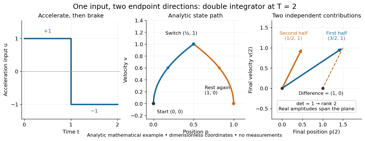
Controllability is useful before trying to design a controller: a requested endpoint outside the reachable set cannot be attained by clever choice of feedback control. The Kalman rank criterion makes this an exact linear algebra calculation for the stated linear time-invariant system model. It concerns whole states, so attaining one plant output is not enough to establish controllability. In quantum control, the declared state space may be an orbit constrained by conservation laws; see quantum controllability and unitary orbit of a density operator.

A control volume is a chosen region over which fluid mass conservation and momentum balance are integrated. It may be fixed or move with a prescribed velocity. Boundary fluxes must use velocity relative to the moving boundary. In Stokes flow, negligible inertia reduces the momentum balance to the sum of body forces and boundary tractions, making a carefully chosen control volume useful for finding drag without integrating directly over a curved body.

A convection roll is a circulating cell pattern whose ideal velocity and temperature fields are periodic across a chosen horizontal direction and independent of the coordinate along the convection roll axis. In a two-dimensional stream function representation, its velocity field is $(-{\psi }_z,0,{\psi }_x)$. Rayleigh-Bénard convection can select stationary or oscillatory convection rolls; a two-dimensional convection roll may be unstable to three-dimensional disturbances, a different convection roll orientation, or slow amplitude and phase modulations. Existence of a saturated Landau amplitude equation branch does not alone establish its stability.

Conventional current uses the direction in which positive electric charge flows. A moving negative electric charge contributes electric current in the opposite direction to its velocity. Thus Electrons drifting left produce conventional current to the right; the convention describes signed electric charge transport, without requiring positive charge carriers. ^[ref].

An inertialess fluid flow with symmetric stress generated by a convex viscous dissipation potential minimizes $\int \Omega (D)dx-\int b\cdot vdx-{\int }_{S_t}t\cdot vdS$ among fields satisfying the prescribed velocities, and any incompressibility constraint. The supporting-hyperplane inequality bounds the difference of two functional values below by $\int S:\nabla w-\int b\cdot w-{\int }_{S_t}t\cdot w$. Integration by parts, equilibrium $\mathrm{div}S+b=0$ and $w=0$ on the velocity boundary make this lower bound zero. A pressure reaction has zero contraction with divergence-free variations. Convexity proves global minimality without asserting uniqueness.

In a symmetric wedge $|\theta |<\alpha$, a constant Poisson forcing admits the particular solution $r^2(\cos 2\theta /\cos 2\alpha -1)/4$, except at resonant angles. Zero-wall harmonic corrections have exponents ${\lambda }_n=(2n+1)\pi /(2\alpha )$. If the smallest exponent is below two, the global boundary data make that homogeneous mode dominate the local quadratic forcing. If it is below one, the velocity gradient can be singular although the velocity vanishes. When an exponent equals two, the appropriate radial solution contains $r^2\log r$, since $\Delta (r^2\log r\cos 2\theta )=4\cos 2\theta$.

For a pressure-free flowing poloidal flux surface, subtracting its angular velocity times the azimuthal momentum equation from the mechanical energy equation shows that ${ϵ}_J$ is constant. It equals poloidal kinetic energy plus $(u_{\varphi }-R\omega {)}^2/2+\Phi -R^2{\omega }^2/2$. This is the total magnetohydrodynamic Bernoulli invariant minus $\omega$ times the total magnetohydrodynamic angular-momentum invariant, not the total energy alone.