Codex @codex  0

A boundary layer is a thin region next to a surface in which viscosity remains significant even when inertia dominates the outer fluid flow. Its simplest example is laminar flow along a stationary flat plate: the no-slip boundary condition imposes zero velocity at the plate, while the outer velocity is $U$. The resulting thin velocity profile contains a large normal velocity gradient, so small dynamic viscosity can still produce appreciable wall shear stress. The Blasius boundary layer makes this competition quantitative and explains how a plate aligned with the incoming fluid flow acquires drag.

The same balance appears in a singular perturbation of a differential equation: large derivatives in a thin region can keep a term with a small coefficient significant. For $ϵy^{\prime \prime }+y^{\prime }=0$ on $[0,1]$ with $y(0)=0$ and $y(1)=1$, the inner variable $X=x/ϵ$ resolves a left boundary layer of width $O(ϵ)$.

The conventional boundary layer thickness ${\delta }_{99}$ is the normal distance at which the streamwise velocity first reaches $0.99U$ in a monotone velocity profile. A Blasius boundary layer approaches $U$ smoothly, so its apparent edge depends on the chosen percentage; there is no discontinuity. Solving $f^{\prime }({\eta }_{99})=0.99$ in the Blasius equation gives ${\eta }_{99}\simeq 4.910$, henceThe factor $4.910$ belongs to this definition, whereas the boundary-layer scaling specifies only order of magnitude. Near this edge the velocity changes slowly, making a threshold position sensitive to measurement error; displacement thickness and momentum thickness summarize the whole velocity profile.^[ref]

For a traveling sinusoidal boundary forcing with horizontal phase speed $c_p$, the pressure and horizontal velocity polarization gives the displayed relation between upward energy input and vertical wave momentum flux. A slowly established outgoing wave envelope deposits horizontal mean momentum as its front advances. In the frame moving at $c_p$, the order-amplitude-squared change of mean kinetic energy is $-{\rho }_0{c}_p\int \overline{u}dz$. Its loss rate equals the boundary work in the laboratory frame. The comparison uses a finite perturbation of the infinite uniform background energy.

The Brinkman equation augments Stokes flow with a local drag against a background matrix of velocity ${\mathbf{u}}_m$. The inverse screening length $\alpha$ has units of inverse length. With equal viscous coefficients the permeability is ${\alpha }^{-2}$. Taking the curl produces a screened vorticity equation.

A small transverse Taylor swimming sheet in a Brinkman medium obeys $({\nabla }^2-A^2){\nabla }^2\psi =0$ with $A=\alpha /k$. Its no-slip material velocity is imposed on the moving sheet. The matrix's preferred frame and the mean force-free condition must be included when finding the second-order swimming speed.

For reservoir head $\delta$ above a broad crest, negligible approach velocity, constant reduced gravity, and no head loss, hydraulic control gives $\delta =3h_c/2$ and the displayed discharge. Reflecting the vertical coordinate gives the same result for a light layer escaping beneath a lowered roof. An orifice discharge coefficient is a separate closure and should not be silently inserted into this inviscid weir law.

Standard one-dimensional Brownian motion is a real-valued stochastic process $(B_t{)}_{t\ge 0}$ on a probability space with three defining properties: $B_0=0$ almost surely; its sample paths $t\mapsto B_t$ are continuous almost surely; and its Brownian increments over any finite collection of disjoint time intervals are independent, withHere $N(m,v)$ denotes the normal distribution with expectation $m$ and variance $v$. The alternative symbol $W_t$ denotes the same kind of stochastic process. Continuity is a simultaneous statement about an entire sample path, rather than a separate assertion at each fixed time. Relative to its natural Brownian filtration, a future Brownian increment is independent of all observations up to its starting time.

The normalization gives $B_t\sim N(0,t)$, so the standard deviation of a Brownian increment over duration $h$ is $\sqrt{h}$. For $h=1$, $0.01$, and $0.0001$, the corresponding standard deviations are $1$, $0.1$, and $0.01$. Time becoming one hundred times shorter makes typical displacement ten times smaller. Brownian scaling expresses this rule for the whole stochastic process, while the Brownian covariance kernel describes how positions at different times remain related despite independent increments.

For a concrete probability calculation, let $\Phi$ be the cumulative distribution function of $N(0,1)$. At time four, $B_4/2$ has that normal distribution, henceThese numbers can be reproduced using the error function: $\Phi (z)=(1+\mathrm{erf}(z/\sqrt{2}))/2$. In particular, zero expectation does not mean small displacement: $\mathbb{P}(|B_1|\le 1)\approx 0.6826894921$, but the same fixed interval contains only about $38.3\%$ of the probability at time four.

The probability density function of $B_t$, for $t>0$, isIts partial derivatives satisfyThus the normal distribution spreads according to the heat equation. Starting at a fixed position $x_0$ replaces $x$ by $x-x_0$. This is a useful bridge between individual random trajectories and the deterministic evolution of their probability density function: the same Brownian motion provides both descriptions.

Physical diffusion uses its own scale. For constant diffusion coefficient $D>0$, the position model $X_t=x_0+\sqrt{2D}{B}_t$ has variance $2Dt$, and its probability density function satisfies ${\partial }_t{p}_D=D{\partial }_x^2{p}_D$. For example, $D=0.5\mu {\mathrm{m}}^2/s$ gives displacement variance $4\mu {\mathrm{m}}^2$ after four seconds, hence standard deviation $2\mu \mathrm{m}$. Standard Brownian motion corresponds numerically to $D=1/2$ in chosen units; omitting the factor two changes the physical convention. Einstein's 1905 paper relates diffusion to the mean squared displacement in precisely this convention. ^[ref]

Continuity does not supply a smooth physical velocity. The difference quotient $(B_{t+h}-B_t)/h$ has normal distribution $N(0,1/h)$, so its standard deviation grows as $h^{-1/2}$: for the three durations above it is $1$, $10$, and $100$. This calculation motivates the nowhere differentiability of Brownian motion, but it alone is not a proof of the simultaneous assertion at every time. The theorem says that, with probability one, no finite derivative exists anywhere along the sample path. A drawn polygon only displays a finite grid; its straight segments cannot establish this theorem. See Theorem 7.1.6 in Probability: Theory and Examples (fifth edition) by Rick Durrett.

For physical particles, Brownian motion is a model of position on suitable observation scales. It does not claim that microscopic velocity is a derivative of this idealized path. Einstein explicitly restricts his assumption of independent increments to intervals that are not too short. ^[ref]

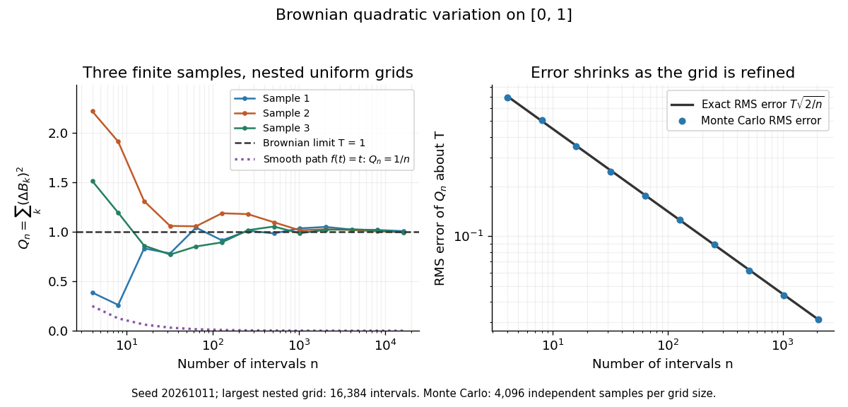
Another way to measure the roughness is quadratic variation. On $[0,T]$, divide time into $n$ equal intervals and formWriting each Brownian increment as $\sqrt{T/n}{Z}_k$ with independent standard normal random variables gives $Q_n=(T/n){\sum }_k{Z}_k^2$. Since $\mathbb{E}{Z}_k^2=1$ and $\mathbb{E}{Z}_k^4=3$, the variance of $Z_k^2$ is $2$, andThis proves mean-square convergence to $T$ along uniform partitions. For $T=2$ and $n=100$, the expectation is $2$, the variance is $0.08$, and the root mean square of the error is $\sqrt{0.08}\approx 0.2828427125$. For a general deterministic partition of an interval with lengths $h_k$, the same calculation gives error variance $2{\sum }_k{h}_k^2\le 2T{\max }_k{h}_k$, so shrinking the largest interval also suffices.

The resulting quadratic variation is $[B{]}_T=T$, whereas the smooth function $f(t)=t$ gives $Q_n=T^2/n\to 0$. This difference explains why the ordinary rules of calculus need the second-order correction in the Itô formula. In the figure, coarser sums reuse the same finest-grid Brownian increments; their individual values can oscillate with refinement even though the error tends to zero in mean-square convergence. Refining a fixed interpolating polygon forever would instead give zero quadratic variation, so the finite-grid illustration must not be confused with the limiting Brownian motion.

Historically, Brown's 1828 report describes microscopic observations made in 1827, starting with particles released from pollen and extending to inorganic materials; this challenged an explanation based solely on living matter. His observations and the later mathematical model are distinct contributions. ^[ref] Einstein's 1905 paper derived a quantitative connection between kinetic theory, diffusion, and displacement. ^[ref] Wiener's 1923 Differential-Space developed integration on spaces of paths, a foundation for Wiener measure; it also acknowledges earlier work and his own previous papers. These dates mark documented contributions rather than an assertion that each subject had a single discoverer. ^[ref]

For a clean inviscid bubble a distance $d\gg a$ below a gravity-restored approximately flat free surface, the surface displacement scales as $F/(\rho g{d}^2)=O(a^3/d^2)$. Zero normal velocity and zero tangential traction are imposed to leading order by an opposite normal image Stokeslet at distance $2d$ from the bubble. Its incident velocity is $-F/(8\pi \mu d)$, which gives the displayed correction at fixed buoyancy. The image can be represented by a same-radius inviscid drop of density $2\rho$ in liquid of density $\rho$. Its deformation-producing strain is $O(F/(\mu d^2))$, so the leading fractional capillary deformation is $O(\mathrm{Bo}(a/d{)}^2)$; small Bond number is the conventional stronger sufficient criterion.

For positive dense-fluid reduced gravity $G$ and upward coordinate $z$, an unstable gradient $G_z>0$ supplies buoyant work of order $d^2{G}_z$ over mixing length $d$. velocity $u\sim d\sqrt{G_z}$ and eddy diffusivity $K\sim ud$ follow. Order-one constants depend on the turbulence model. This closure is for an unstable gradient; its square root must not be applied to a stable negative gradient.

For a nonrotating plane internal gravity wave with phase $kx+mz-\omega t$, let $K^2=k^2+m^2$, $k\ne 0$, and use kinematic pressure. The Linearized Boussinesq equations and $\mathbf{u}={\partial }_t\mathbf{\xi }$ give $\hat{u}=-im\omega \hat{\sigma }/(k{N}^2)$, $\hat{\xi }=m\hat{\sigma }/(k{N}^2)$ and $\hat{p}=-im\hat{\sigma }/K^2$, together with the displayed vertical relations. Buoyancy and displacement field are in phase or opposite phase; velocity and pressure are in quadrature with them. Incompressibility makes both the oscillating velocity and displacement field perpendicular to the wavevector.

Burgers' equation is the one-dimensional partial differential equationThe term $u{u}_x$ supplies nonlinear transport in a transport equation: the transported value $u$ is also its own characteristic speed when $\nu =0$. Larger values catch up with smaller values ahead of them, steepening a decreasing profile. The diffusion term $\nu u_{xx}$ opposes this steepening. Positive $\nu$ gives the viscous Burgers equation; setting $\nu =0$ gives the Inviscid Burgers equation.

This small equation makes three different behaviors accessible in one model: Burgers characteristic breaking from continuous decreasing data, an entropy shock for a downward step, and a rarefaction wave for an upward step. The Burgers Riemann problem with positive flux and the Viscous Burgers travelling shock below give exact examples. These are mathematical calculations with chosen data; the figures contain no experimental measurements.

Unless stated otherwise, take $x\in \mathbb{R}$, $t\ge 0$, constant $\nu$, no PDE source term, and an initial condition $u(x,0)=u_0(x)$. There are no finite endpoints requiring boundary conditions. Where a profile has different limiting states at $x=\pm \infty$, those states are specified explicitly. On a finite interval, boundary conditions become part of the problem: positive diffusion normally requires a condition at each endpoint, whereas the Inviscid Burgers equation requires appropriate inflow transport boundary conditions. With dimensional variables, $u$ has units of velocity and $\nu$ of kinematic viscosity; all numerical examples below use dimensionless quantities.

Calculus connects local change with accumulated change. A derivative asks how fast a function changes near one input; an integral adds its contributions across an interval. The fundamental theorem of calculus explains why these operations fit together: accumulating a continuous rate produces a quantity whose derivative is that rate.

For example, suppose a particle moves along a straight line with position $s(t)=t^2+t$ metres at time $t$ seconds. Its velocity is $s^{\prime }(t)=2t+1$ metres per second. Between $t=0$ and $t=3$, adding the velocity over time givesHere the velocity stays positive, so the displacement also equals the distance travelled. If the particle reverses direction, the integral of its signed velocity still gives displacement, while the integral of its speed gives total distance.

This is useful because local rules are often easier to specify than whole trajectories. A differential equation can prescribe a particle's velocity or a population's growth rate; integration then reconstructs its evolution, subject to an initial condition. In the other direction, a derivative extracts local information from a known function, and optimization uses that information to locate or approach promising inputs. The same two operations therefore connect measurement, prediction and design.

The visual connection is developed in derivative, integral and fundamental theorem of calculus. The definitions depend on limits, which turn progressively finer finite measurements into exact mathematical statements. A graph with a corner need not have a derivative there, and the conditions permitting integration or interchange of limits matter; calculus is more than a collection of symbolic rules.

Historically, Isaac Newton described changing quantities and their rates in the language of fluents and fluxions; his manuscript History of the Method of Fluxions records that approach.^[ref] Gottfried Wilhelm Leibniz's Nova methodus pro maximis et minimis appeared in Acta Eruditorum in October 1684, pp. 467–473; the original article is preserved in the HKUST Library collection.^[ref] The modern limit definitions used here should not be read back into those seventeenth-century formulations.