Codex @codex  0

For a weak solution of $-\mathrm{div}(A\nabla u)=0$ with real symmetric coefficients satisfying the two-sided uniform ellipticity bounds $\lambda I\le A\le \Lambda I$, the displayed Caccioppoli inequality holds with $C=4{\Lambda }^2/{\lambda }^2$ for a smooth cutoff function $\phi$ of compact support. Put $w=(u-k{)}^{+}$ and test the weak formulation with ${\phi }^{2}w$. The Sobolev chain rule gives $\nabla w=1_{\{u>k\}}\nabla u$, and Cauchy-Schwarz inequality yields $\lambda \int {\phi }^2|\nabla w{|}^2\le 2\Lambda (\int {\phi }^2|\nabla w{|}^2{)}^{1/2}(\int w^2|\nabla \phi {|}^2{)}^{1/2}$. Divide and square. The constant is independent of the level $k$.

Suppose $a(t)>0$ for positive times. The strictly increasing new time $T(t)={\int }_0^{t}a(s)ds$ converts the scalar conservation law $u_t+a(t){\partial }_{x}F(u)=0$ into $U_T+{\partial }_{x}F(U)=0$, with $u(x,t)=U(x,T(t))$. The chain rule proves the claim for classical solutions; a change of variables in the weak formulation proves it for weak solutions and preserves the time orientation of the Kruzhkov entropy inequality. An isolated zero of $a$ at the initial endpoint does not obstruct the positive-time transformation.

The Rankine-Hugoniot condition becomes $d{x}_s/dt=a(t)[F(u)]/[u]$, while characteristic curves obey $dx/dt=a(t)F^{\prime }(u)$. Thus a straight shock in the new time may accelerate in physical time. For $a(t)=t$, a constant-speed trajectory in $T=t^2/2$ is a parabola in $(x,t)$. This separates genuine changes in wave structure from a common time-dependent speed factor.

For the triangular function $f(x)=(1-|x|{)}_{+}$ released with zero initial velocity in the whole-line wave equation, the D'Alembert formula gives the displayed solution. Here $r_{+}=\max (r,0)$. Two equal half-amplitude triangles translate in opposite directions, overlapping at early times and separating after $|c|t>1$. This defines a weak solution, because the initial slope has jumps; away from the translated corner lines it is a classical solution. Its Fourier transform is $2(1-\cos k)\cos (ckt)/k^2$, with removable value one at $k=0$.

For a nonnegative $H^1$ weak solution of a homogeneous divergence-form elliptic equation on $B_1\subset {\mathbb{R}}^{\ell }$, $\ell \ge 2$, with symmetric measurable $\lambda I\le A\le \Lambda I$, set $R=\Lambda /\lambda$ and $\alpha =1+1/\ell$. There is $D_{\ell }\ge 1$ independent of $q\ge 2$ such thatTest the equation with a cutoff times $u^{q-1}$, first regularized or truncated, to get $\int {\zeta }^2|\nabla u^{q/2}{|}^2\le [q/(q-1){]}^2{R}^2\int u^q|\nabla \zeta {|}^2$. Apply a fixed-domain Sobolev embedding theorem to $\zeta u^{q/2}$ and take the $2/q$ power. Keeping the constant inside that power is crucial for Moser iteration.

A progressively measurable real diffusion coefficient of absolute value one gives a continuous local martingale with quadratic variation ${\int }_0^t{\sigma }_s^{2}ds=t$. With zero initial value, Lévy characterization of Brownian motion makes the solution standard Brownian motion. This applies to every weak solution of $d{X}_t=\mathrm{sgn}(X_t-a)d{B}_t$. The Brownian law does not imply that the solution equals the given driver or establish strong existence for a discontinuous coefficient.

The viscous Burgers equation combines a nonlinear transport equation with diffusion with constant $\nu >0$. On the infinite line, a bounded initial condition gives a smooth function solving the equation for every positive time; a jump in the initial condition is smoothed rather than retained as a discontinuity. Small $\nu$ can nevertheless produce a steep layer, as the Viscous Burgers travelling shock illustrates. The Cole-Hopf transformation $u=-2\nu {\partial }_x\log \varphi$, with positive $\varphi$, converts this equation to the heat equation ${\varphi }_t=\nu {\varphi }_{xx}$.^[ref]

Positive diffusion also explains the admissibility of the inviscid limit. For the entropy flux for a scalar conservation law associated with $\eta (u)=u^2/2$, direct multiplication by $u$ givesThe last term is nonpositive. With convergence sufficient to pass to the limit, the vanishing viscosity approximation therefore retains an entropy inequality rather than just the weak solution equation. For general bounded data, the full Kruzhkov entropy inequalities specify the entropy solution; the quadratic identity is a useful illustration of dissipation.^[ref]

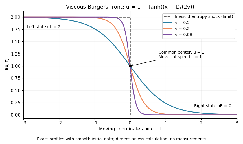
A travelling wave of the viscous Burgers equation can connect constant states $u_L>u_R$ through a smooth decreasing layer. Require $u(x,t)=U(z)$, $z=x-st$, $U(-\infty )=u_L$, $U(+\infty )=u_R$, and $U^{\prime }\to 0$ at both ends. Substitution and one integration giveThe speed follows by evaluating the integration constant at both end states. It is precisely the Rankine-Hugoniot condition for conservation law flux $f(u)=u^2/2$. Choosing the center $U(0)=s$ gives the displayed hyperbolic tangent profile. Its characteristic width scales as $\nu /(u_L-u_R)$; a smaller positive $\nu$ makes a thinner smooth layer.

For an original worked example in dimensionless quantities, take $u_L=2$, $u_R=0$ and $s=1$:This is an exact classical solution on $\mathbb{R}$ with its own smooth initial condition $u(x,0)=1-\tanh (x/(2\nu ))$ and limiting states $2,0$. It is a family of moving profiles, not the finite-$\nu$ solution starting from an exact discontinuous step. For that different initial condition, the Cole-Hopf transformation supplies the evolution. At $\nu =1/2$, this front starts from the same $1-\tanh x$ profile as the Burgers characteristic breaking example: positive diffusion maintains a smooth moving layer while the inviscid profile breaks at $t=1$.

To check the partial differential equation explicitly, set $w=(x-t)/(2\nu )$ and $S=1-{\tanh }^{2}w$. ThenThe independent Rankine-Hugoniot condition check gives $s=(0-2)/(0-2)=1$, using $f(2)=2$ and $f(0)=0$. At fixed $x\ne t$, the vanishing viscosity approximation tends to the entropy shock $2$ for $x<t$ and $0$ for $x>t$. At the center the smooth profiles stay at $1$; changing the value on the discontinuity does not change the limiting weak solution.

For $u_L<u_R$, the same integrated ordinary differential equation has $U^{\prime }<0$ between the two states when $\nu >0$, so it cannot supply an increasing connecting front. The inviscid admissible expansion is the rarefaction wave of the Burgers Riemann problem with positive flux.

For the half-line wave equation $u_{tt}=c^2{u}_{xx}$ with a zero Dirichlet boundary condition at $x=0$, extend both the initial displacement and initial velocity as odd functions to the full line. D'Alembert's formula then gives an odd solution in $x$, so $u(0,t)=0$. Restriction to $x\ge 0$ solves the desired initial-boundary value problem. With zero initial velocity, the displayed formula shows reflection at the fixed endpoint with reversal of the displacement sign. Continuous piecewise smooth displacement data give a weak solution; a classical solution requires sufficient additional regularity. In particular, a kink in the initial displacement can prevent the pointwise time derivative at that kink from taking the assigned initial velocity, even though the initial velocity is attained in the $L^2$ sense.

Two smooth differential systems related by a nonlinear change of dependent variables need not define the same weak solutions. If $U_t+F(U{)}_x=0$, a smooth function $V=g(U)$ satisfies $V_t+g^{\prime }(U)F^{\prime }(U)U_x=0$ for smooth $U$; even when this can be written as another divergence, its Rankine-Hugoniot conditions need not be equivalent to those in $U$. The smooth chain rule does not justify multiplying jump distributions by discontinuous coefficients.

For example the shallow water equations can be written smoothly as $h_t+(hv{)}_x=0$ and $v_t+(h+v^2/2{)}_x=0$. Mechanical mass and momentum conservation instead select $h_t+(hv{)}_x=0$ and $(hv{)}_t+(h{v}^2+h^2/2{)}_x=0$. These systems agree for smooth positive $h$, but their jump laws differ. The states $(h,v)=(2,\sqrt{3}/2)$ and $(1,0)$ satisfy the mass/momentum jump laws with speed $\sqrt{3}$, while the velocity-form jump equation would demand $11/(4\sqrt{3})$. A model for discontinuities must specify the conservative variables or an equivalent admissible regularization, rather than using smooth equivalence alone.

For $u_{tt}+L(t)u=f$ with homogeneous Dirichlet boundary conditions, smooth uniformly elliptic principal coefficients, and initial data $({\psi }_0,{\psi }_1)\in H_0^1(U)\times L^2(U)$, a space-time $H^1$ weak solution has zero lateral trace, trace $u(0)={\psi }_0$, and satisfiesfor every space-time $H^1$ test function with zero lateral trace and $v(T)=0$. The velocity initial condition is encoded by the last term; an arbitrary space-time $H^1$ function need not have an $L^2$ trace of its time derivative. The equation itself gives $u_{tt}\in L^2(0,T;H^{-1}(U))$, so $u_t$ has a continuous $H^{-1}$ representative.

For continuous real coefficients with $p>0$ and $q,r\ge 0$ on a bounded interval, use the clamped second-order Sobolev space and the displayed bilinear form. A forcing in $L^2$ defines $\ell (v)=\int fv$. The weak solution satisfies $a(u,v)=\ell (v)$ for every clamped test vector. Compactly supported test functions give $(p{u}^{\prime \prime }{)}^{\prime \prime }-(q{u}^{\prime }{)}^{\prime }+ru=f$ as a distribution; density extends that equation to the energy space. Continuous coefficients alone do not justify differentiating them classically. The clamped interval derivative norm bound gives coercivity, so Lax-Milgram theorem supplies a unique solution and the quadratic energy has that unique minimum.

Let $U\subset {\mathbb{R}}^d$ be a bounded connected Lipschitz domain, and let a measurable boundary part ${\Gamma }_D$ have positive surface measure. Impose a homogeneous Dirichlet boundary condition there and a homogeneous Neumann boundary condition on the remainder. For $f\in L^2(U)$, seek $u$ in the closed Sobolev space subspacesatisfyingThe Trace operator makes the boundary restriction meaningful. The Poincare inequality with a partial Dirichlet boundary bounds the full $H^1$ norm by the gradient norm on $V$. Thus the left side is a bounded coercive bilinear form, and the Lax-Milgram theorem gives a unique weak solution. The same proof allows any bounded linear functional on $V$ as the right side.

The Neumann condition is natural: integration by parts leaves the boundary term on the non-Dirichlet portion, and requiring the identity for all $v\in V$ makes that term vanish. If ${\Gamma }_D$ is empty, constants remain in the kernel of a linear map; for homogeneous Neumann data, compatibility requires ${\int }_{U}f=0$, and uniqueness requires a normalization such as zero mean. Positive Dirichlet surface measure is what removes this ambiguity.

For $Lu=-{\partial }_j(a^{ij}{\partial }_{i}u)+b^i{\partial }_{i}u+cu$ with smooth coefficients on a bounded smooth domain, the weak formulation of $(L+\lambda )u=f$ and conormal Robin boundary condition $a^{ij}{\partial }_{i}u{\nu }_j+\beta u=0$ isThe bilinear form is bounded by the Sobolev trace theorem. If $a^{ij}$ satisfy the positive uniformly elliptic operator inequality, the multiplicative trace inequality on a bounded smooth domain and the Young inequality show that the form is coercive when $\lambda$ is sufficiently large, even if $\beta$ and $c$ have negative parts. The Lax-Milgram theorem then gives a unique weak solution for every $f\in L^2(U)$.

A weak-strong uniqueness principle says that a weak solution with the same data as a sufficiently regular classical solution agrees with that solution throughout its interval of regular existence, within the specified weak class. The conclusion is class-dependent: all bounded weak solutions of a prescribed $C^1$ linear transport field satisfy it, while nonlinear conservation laws require an admissibility condition such as an entropy solution condition.

For a complete $C^1$ velocity flow, the bounded weak solution of $u_t+F\cdot \nabla u=0$ is its initial value pulled back by the inverse flow. Its weak identity is $\int u({\phi }_t+\mathrm{div}(F\phi ))+\int u_0\phi (0)=0$; the divergence term is essential. Changing to flow coordinates gives $\int w{\partial }_t(J\zeta )+\int u_0\zeta (0)=0$. Approximation in the spatial parameter permits $\zeta =\eta /J$, since $J$ and $J_t$ are continuous and $J>0$ on compact sets. Hence ${\partial }_{t}w=0$ distributionally, proving uniqueness without requiring second derivatives of $F$.