Codex @codex  0

Fix $u_l>u_r$ and the Rankine-Hugoniot condition speed from the preceding part. The new hypothesis is a uniformly convex scalar flux, $F^{\prime \prime }\ge \kappa >0$; it replaces the globally bounded-$F^{\prime }$ hypothesis of part (a). Choose $b=\sigma u_r-F(u_r)$. Thensince a strictly convex function lies below the chord between its two endpoint values. Also $Q(u_l)=Q(u_r)=0$ andThe zeros at the endpoints are simple, so the separated integral diverges logarithmically there. Thus the travelling wave is a decreasing connection defined for all $s$, unique up to translation.

To specify a limit, fix a number $c\in (u_r,u_l)$ independently of $\epsilon$ and normalize $v_{\epsilon }(0)=c$. If $V^{\prime }=Q(V)$ and $V(0)=c$, uniqueness gives $v_{\epsilon }(s)=V(s/\epsilon )$. ConsequentlyAt $x=\sigma t$ the normalized profile equals $c$ for every $\epsilon$. This single-line value is immaterial to the weak solution. Convergence holds pointwise off the line and in $L_{\mathrm{loc}}^1$ by bounded convergence; it cannot be uniform across a nonzero jump. The transition has thickness of order $\epsilon$.

This is the vanishing viscosity approximation to a compressive entropy shock. The Rankine-Hugoniot condition makes the step a weak solution of the inviscid scalar conservation law, while $F^{\prime }(u_r)<\sigma <F^{\prime }(u_l)$ means characteristic curves enter the shock from both sides. For every smooth convex function $\eta$ used as an entropy, with entropy flux for a scalar conservation law $q^{\prime }={\eta }^{\prime }{F}^{\prime }$, the viscous equation givesAgainst compactly supported tests the right side tends to zero, since $u_{\epsilon }$ stays in $[u_r,u_l]$. Passing to the $L_{\mathrm{loc}}^1$ limit yields the entropy inequality, explaining the direction selected by positive viscosity.

A translation must be fixed to obtain this particular limit. An $\epsilon$-dependent translate $V((s-a_{\epsilon })/\epsilon )$ can converge to a shock at a different location, to a constant if its center escapes, or fail to converge if the centers oscillate. Thus existence of profiles alone does not specify a single vanishing-viscosity limit without a phase normalization.

Write the negative-flux Inviscid Burgers equation as $f_Z+{\partial }_{\theta }F(f)=0$, with $F(f)=-f^2/2$. Along a characteristic curve,so a characteristic starting at ${\theta }_0$ has $\theta ={\theta }_0-f_0({\theta }_0)Z$ andThis formula is a classical solution only while the method of characteristics is one-to-one; after characteristic crossing one must select an entropy solution.

For a discontinuity with left and right values $f_{-}$ and $f_{+}$, the Rankine-Hugoniot condition follows by integrating conservation across a moving small interval:For a nonzero jump, factor the difference of squares to obtainThe negative flux makes increasing jumps compressive. Decreasing jumps spread into rarefaction waves; they cannot be retained as nonphysical expansion shock waves.

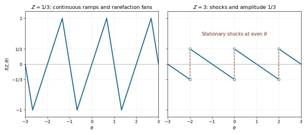
In the central ramp of each period, $f_0({\theta }_0)={\theta }_0-2m$, so its method of characteristics is $\theta -2m=(1-Z)({\theta }_0-2m)$. For $0<Z<1$, the retained ramp therefore occupies $|\theta -2m|<1-Z$. At the odd boundary $r=2m+1$, the initial limiting values are $+1$ on the left and $-1$ on the right. Their characteristic speeds are $-1$ and $+1$, giving the fan $f=-(\theta -r)/Z$ on $|\theta -r|<Z$. Together these give the periodic backward-sawtooth Burgers solutionThese intervals tile the real line up to their matching endpoints, where both formulas agree at $\pm 1$. The increasing ramp steepens, but the wave's maximum magnitude remains one before breaking. A steep continuous regularization of the original downward jump produces exactly the limiting fan, as suggested by the characteristic construction.

At $Z=1$, each increasing ramp collapses at $\theta =2m$. The fans on either side meet there with values $-1$ and $+1$, producing a compressive stationary shock wave. For all $Z\ge 1$ the fan between successive shock waves remains centered at the odd point, givingAt a shock wave the limiting values are $f_{-}=-1/Z$ and $f_{+}=1/Z$. Their average is zero, so the Rankine-Hugoniot condition keeps the shock wave fixed. Their characteristic speeds satisfy $1/Z>0>-1/Z$, confirming compression into the shock wave. The arbitrary pointwise value at a shock wave does not affect the weak solution. The post-breaking amplitude decays as $1/Z$, despite the lack of explicit viscosity, because shock wave dissipate the wave.

For the requested sketches, $Z=1/3$ has ramp slope $3/2$ on $|\theta -2m|<2/3$ and fan slope $-3$ around odd points on width $2/3$. It is still continuous. At $Z=3$, the profile decreases linearly with slope $-1/3$ between even points and jumps from $-1/3$ to $+1/3$ at each even point:

A weak solution is an equivalence class $u\in L^{\infty }((0,\infty )\times \mathbb{R})$ satisfying, for every test function $\phi \in C_c^{\infty }([0,\infty )\times \mathbb{R})$,This is integration by parts for the nonconservative transport equation. In particular, the weak formulation contains $c_x\phi$ as well as $c{\phi }_x$. The last integral encodes the initial condition; a pointwise boundary value of an arbitrary Lebesgue space representative is not the definition. Compact support of the test function makes the identity meaningful even if $c$ is unbounded.

Use the same formula for a measurable representative of $u_0$. Dilation preserves null sets and gives $\Vert u{\Vert }_{L^{\infty }}=\Vert u_0{\Vert }_{L^{\infty }}$. To check the weak formulation, change variables $x=e^{t}y$ and set $\psi (t,y)=e^t\phi (t,e^{t}y)$. ThenThe spacetime integral becomes $\int u_0(y){\psi }_t(t,y)dydt=-\int u_0(y)\phi (0,y)dy$, as required.

For uniqueness, take any bounded weak solution and write $v(t,y)=u(t,e^{t}y)$. Choosing $\phi (t,x)=e^{-t}\psi (t,e^{-t}x)$ in the weak formulation givesFor tensor test functions $\psi (t,y)=\eta (t)\theta (y)$, this says that $\int v(t,y)\theta (y)dy$ is distributionally constant and has value $\int u_0\theta$. A countable dense family of spatial test functions identifies $v=u_0$ almost everywhere. Thus the displayed solution is the unique bounded weak solution.

A characteristic curve has $x-at$ constant. Backtracking reaches the initial line if $x\ge at$ and the inflow boundary otherwise. HenceValues on the dividing characteristic curve are immaterial for bounded weak solutions.

For a classical solution on the closed quadrant, choose $u_0,f\in C^1([0,\infty ))$ and impose the corner compatibility for constant-speed transportThese make the values and both first derivatives agree across $x=at$; each branch solves the transport equation. They are also necessary for a $C^1$ solution up to the initial and inflow boundaries.

Spatial $C^{\infty }$ regularity for every $t\ge 0$, up to $x=0$, holds precisely for smooth data with all matching jets:Indeed the spatial derivatives of order $n$ at $x=at$ are $u_0^{(n)}(0)$ and $(-1/a{)}^n{f}^{(n)}(0)$. Necessity of smooth $u_0$ follows at $t=0$; smoothness of $f$ on any finite interval follows by reading the boundary branch in a spatial slice at a larger time.

For the inflow transport boundary condition, the weak formulation isHere $\phi$ is a smooth compactly supported test function on the closed quadrant. Put $z=x-at$ and $\psi (t,z)=\phi (t,z+at)$. The transformed region is $t>\tau (z):=\max (0,-z/a)$. The formula in the preceding solution is $v(t,z)=b(z)$, with $b(z)=u_0(z)$ for $z\ge 0$ and $b(z)=f(-z/a)$ for $z<0$. Consequently the first integral equals $-\int b(z)\psi (\tau (z),z)dz$. Its positive-$z$ portion cancels the initial integral; the substitution $z=-at$ in its negative-$z$ portion cancels the inflow integral, including the factor $a$. This proves weak existence for arbitrary bounded data without corner compatibility.

For uniqueness, subtract two weak solutions. Interior test functions in these characteristic coordinates give ${\partial }_{t}v=0$ distributionally, so $v(t,z)=b(z)$ on each vertical ray. This follows first on rectangles compactly contained in $t>\tau (z)$ using tensor test functions, and then on the whole region by overlapping rectangles. In the full weak formulation the remaining lower-boundary term is $-\int b(z)\psi (\tau (z),z)dz=0$. Arbitrary smooth traces supported separately on $z>0$ and $z<0$ force $b=0$ there. The single point $z=0$ has zero measure. Thus the two-branch formula is the unique bounded weak solution.

Choose a fixed smooth cutoff function with $\Vert {\zeta }^{\prime }{\Vert }_{\infty }=C_0$ and set $J=(-1/2,1/2)$. The Caccioppoli inequality gives $\Vert u^{\prime }{\Vert }_{L^2(J)}\le 2R{C}_0\Vert u{\Vert }_{L^2(-1,1)}$. Since the length of $J$ is one, the corrected interval Sobolev supremum estimate yields $\Vert u{\Vert }_{L^{\infty }(J)}\le \Vert u{\Vert }_{L^2(J)}+\Vert u^{\prime }{\Vert }_{L^2(J)}$, and the Hölder seminorm is at most $\Vert u^{\prime }{\Vert }_{L^2(J)}$. ThereforeFor locally $H^1$ weak solutions with $u\in L^2(-1,1)$, density of smooth functions in a Sobolev space justifies the test ${\zeta }^{2}u$, and the previous representative estimates already apply to $H^1$. Mollifying a solution need not preserve the equation with the same measurable coefficient, so approximation is used for admissible tests and Sobolev estimates, not to assert that the mollified function solves the original equation. The required constant depends only on $R$.

For a real weak solution $u\in H_{\mathrm{loc}}^1(B_1)$, $\int A\nabla u\cdot \nabla \varphi =0$ for compactly supported $H^1$ tests. The symmetric coefficient bounds give $A\xi \cdot \xi \ge \lambda |\xi {|}^2$ and $|A\xi |\le \Lambda |\xi |$. Test with $\varphi ={\zeta }^{2}u$ and apply the Cauchy-Schwarz inequality:Thus $E\le 4R^{2}I$, including $E=0$. As $\zeta =1$ on $B_{r_1}$ and has support in $B_{r_2}$,This Caccioppoli inequality is valid for smooth solutions and, by density of admissible tests, for locally $H^1$ weak solutions with bounded measurable coefficients.

The original PDF assumes $u\ge 0$ at the beginning of this question; the TeX conversion omits that hypothesis. First replace a smooth nonnegative solution by $v=u+\epsilon >0$, which solves the same homogeneous divergence-form elliptic equation. For $w=v^{q/2}$, the chain rule gives the favorable termin the distributional sense. Thus $w$ is a weak subsolution. Testing its subsolution inequality with ${\zeta }^{2}w$ yields the same Caccioppoli inequality as before. More precisely, testing the equation for $v$ with ${\zeta }^2{v}^{q-1}$ givesIndeed the main term is at least $(q-1)\lambda \int {\zeta }^2{v}^{q-2}|\nabla v{|}^2$, and the cross term is bounded by twice $\Lambda$ times the square roots of this weighted gradient integral and $\int v^q|\nabla \zeta {|}^2$. Let $\epsilon \downarrow 0$ to obtain the stated power energy estimate.

Apply the fixed-domain Sobolev embedding theorem to $\zeta u^{q/2}$. The crucial constant stays uniform before taking the $2/q$ power:where $D_{\ell }\ge 1$ is independent of $q$. This is uniform power gain for elliptic solutions. The exponent is $q\alpha$, not the TeX conversion's $q^{\alpha }$. The PDF's weaker prefactor $C_{\ell }$ outside the $2/q$ power follows from this stronger estimate, but that weaker form alone cannot be iterated infinitely.

For completeness, the estimate also extends to nonnegative locally $H^1$ weak solutions without assuming they are already bounded. For $s\ge 0$ define $F_M(s)=s^{q/2}$ up to $M$ and continue it linearly with slope $(q/2)M^{q/2-1}$ above $M$; set ${\Psi }_M(s)={\int }_0^s{F}_M^{\prime }(r{)}^{2}dr$. Both have bounded derivatives for fixed $M$. Direct calculation gives ${\Psi }_M/F_M^{\prime }\le F_M$ and $F_M(s)\le (q/2)s^{q/2}$. Test the weak equation with ${\zeta }^2{\Psi }_M(u)$, using smooth approximations to these Sobolev chain rule functions if needed. The resulting weighted energy bound is $\int {\zeta }^2|\nabla F_M(u){|}^2\le 4R^2\int F_M(u{)}^2|\nabla \zeta {|}^2$. If $u\in L^q(B_{r_2})$, dominated convergence on the right and the Fatou lemma on the Sobolev left give the boxed gain as $M\to \infty$, with the same uniform constant. Starting with $q=2$, this justifies every subsequent iteration step.

Set $q_i=2{\alpha }^i$, $r_i=1/2+2^{-i-1}$ and $N_i=\Vert u{\Vert }_{L^{q_i}(B_{r_i})}$. Then $r_0=1$, $r_i-r_{i+1}=2^{-i-2}$, and the sharper uniform power gain for elliptic solutions givesThe Moser product on geometric radii converges becauseThus every $N_i$ is at most $B=(D_{\ell }R{)}^{S_0}{2}^{S_1}\Vert u{\Vert }_{L^2(B_1)}$. Since $B_{1/2}\subset B_{r_i}$, its $L^{q_i}$ norms are also bounded by $B$. If $u>B+\delta$ on a set of positive measure $m$ in $B_{1/2}$, these norms are at least $(B+\delta )m^{1/q_i}$, tending to $B+\delta$, a contradiction. HenceThis is the required Moser iteration estimate, with a finite constant depending only on $\ell$ and $R$. The weak-test truncation argument in the preceding solution makes the conclusion valid for locally $H^1$ weak solutions with $u\in L^2(B_1)$ and measurable uniformly elliptic coefficients. No differentiability of $A$ or unproved smooth approximation of solutions is required.

There is a genuine conflict in the printed coefficient assumptions: no uniformly positive coefficient in a zero-boundary Sobolev space exists. A function $a\in H_0^1(\Omega )$ cannot also obey $a\ge a_{-}>0$ almost everywhere. Indeed, the Lipschitz truncation $g(s)=\min (\max (s,0),a_{-})$ has $g(0)=0$, so Lipschitz truncation preserves zero-boundary Sobolev spaces, giving $g(a)\in H_0^1(\Omega )$. But $g(a)$ would be the nonzero constant $a_{-}$. Its zero gradient contradicts the Poincaré inequality in the zero-boundary Sobolev space. Thus the literal coefficient class is empty.

For the meaningful uniformly elliptic problem, take $a\in L^{\infty }(\Omega )$ with $0<a_{-}\le a\le a_{+}$, and impose the Dirichlet boundary condition on the unknown and test functions: $V=H_0^1((0,1{)}^2)$. Additional $H^1$ regularity of $a$ is harmless, but a zero trace for $a$ must be removed. The divergence-form elliptic operator is $L=-\mathrm{div}(a\nabla )$. Integration by parts defines the symmetric bounded bilinear formIn particular,Here $2{\pi }^2$ is the first Dirichlet Laplacian eigenvalue on the unit square; the Poincaré inequality follows, for example, by applying the one-dimensional inequality in each coordinate and adding. Thus $B$ is coercive in the gradient norm on $V$, and the Dirichlet realization of $L$ is a positive definite symmetric operator. On its operator domain, $⟨Lv,v⟩=B(v,v)$.

The required functional and weak equation areBecause $f\in L^2$, the right side is a bounded linear functional by the Cauchy-Schwarz inequality and Poincaré inequality. The Lax-Milgram theorem gives a unique weak solution, and part (b) proves that it uniquely minimizes $I$. These formulas prove the intended conclusion under the repaired coefficient hypothesis; under the literal hypothesis there is no coefficient to which the conclusion can be applied.

Use a Lipschitz continuous cutoff function $\eta$ which equals one on $B_R(x_0)$, vanishes outside $B_{2R}(x_0)$, takes values in $[0,1]$, and has $|\nabla \eta |\le 2/R$. Its gradient is supported in the annulus $A_R=B_{2R}(x_0)\setminus B_R(x_0)$. The function ${\eta }^2(u-c)$ is an admissible test function in the zero-boundary Sobolev space for the weak solution, by approximation with smooth compactly supported test functions. If ${\Lambda }_0$ bounds the operator norm of $(a^{ij})$, we can take ${\Lambda }_0=n\Lambda$. The weak equation and uniform ellipticity giveYoung inequality bounds the right side byAfter absorption, this annular Caccioppoli inequality isThe dimension is fixed in the notation $C(\lambda ,\Lambda )$ of the question; with the entrywise coefficient bound its dependence on $n$ is absorbed there. If the larger ball merely lies in $B$ without its closure being compactly contained, approximation from smaller cutoff functions gives the same admissible test function and estimate. Crucially, the right side uses only the annulus, where the cutoff function varies. The constant $c$ is arbitrary because constants have zero gradient.

The Neumann boundary conditions select the spatial eigenfunctions $\cos nx$, $n=0,1,\dots$, of the separated wave equation. Indeed separation gives $X^{\prime \prime }+\lambda X=0$ with $X^{\prime }(0)=X^{\prime }(\pi )=0$. Integration by parts gives $\lambda \int X^2=\int X^{\prime 2}\ge 0$. The zero value yields the constant mode; for positive $\lambda$, the first boundary condition removes the sine term and the second requires $\sqrt{\lambda }=n\in \mathbb{N}$. For $n>0$, the temporal factor is $\cos nct$: the sine factor vanishes because the initial velocity is zero. The zero mode has constant displacement, with no term linear in time for the same reason.

The constant Fourier cosine series coefficient is the mean ${\pi }^{-1}{\int }_0^{\pi }bxdx=b\pi /2$. The remaining coefficients areOnly odd modes survive. Thus the displacement isThe series for displacement converges absolutely and uniformly. The initial velocity is zero in the finite-energy sense, and the initial displacement is $bx$. There is an endpoint compatibility qualification: when $b\ne 0$, the initial slope does not satisfy the Neumann boundary conditions at $t=0$. The answer is therefore a finite-energy weak solution, piecewise classical between the propagating corners, rather than a globally twice continuously differentiable solution up to the initial endpoints. The mode expansion implements reflection at those endpoints.

Work with real-valued functions. The screened sine-Gordon energy is well defined: $0\le 1-\cos u\le u^2/2$, and $fu$ is integrable by the Cauchy-Schwarz inequality. It is coercive, becauseA minimizing sequence is bounded in the Hilbert space $H^1$. Weak sequential compactness of bounded sequences in a reflexive Banach space supplies a weakly convergent subsequence. The squared H1 space norm is weakly lower semicontinuous, the source pairing is weakly continuous, and the nonlinear term is covered by local Sobolev compactness gives lower semicontinuity of a nonnegative integral. The direct method in the calculus of variations therefore gives a minimizer $\varphi$.

Taking its first variation in any $v\in H^1$ givesThus the Euler-Lagrange equation isas a weak solution, equivalently in distributions when tested against smooth compactly supported functions. The derivative of the nonlinear term is justified by $|\sin \varphi |\le |\varphi |$ and the second-order remainder bound $|\cos |\le 1$.

Now $G=f-\sin \varphi \in L^2$, so the supplied elliptic regularity estimate puts $\varphi$ in $H^2$. Applying the Sobolev inequality to $\varphi$ and each first weak derivative gives $\varphi \in W^{1,6}({\mathbb{R}}^3)$. Morrey's inequality and uniformly continuous integrable functions vanish at infinity prove that its continuous representative tends to zero.

The final printed supremum estimate is false in general. The maximum bound for a monotone reaction term involves $h(s)=s+\sin s$, which is odd and strictly increasing: $h^{\prime }=1+\cos s\ge 0$, and its zeros are isolated. If $M=\Vert f{\Vert }_{\infty }<\infty$, a positive maximum $m$ of $\varphi$ satisfies $h(m)\le f\le M$; apply the same argument to $-\varphi$. The valid general estimate isThe bound by $M$ is valid if $M\le \pi$, but $h(s)$ can be smaller than $s$ for larger positive $s$.

For an explicit failure of the source-size bound for the screened sine-Gordon equation, take $a=3\pi /2$, $L=10$, $\varphi (x)=a{e}^{-|x{|}^2/L^2}$ and $f=-\Delta \varphi +\varphi +\sin \varphi$. These are smooth functions in the required spaces. With $q=|x{|}^2/L^2$,Hence $\Vert f{\Vert }_{\infty }\le a-1+6a/L^2<a=\Vert \varphi {\Vert }_{\infty }$. Moreover $V(s)=s^2/2+1-\cos s$ has $V^{\prime \prime }=1+\cos s\ge 0$, so the energy is convex and this critical point is a minimizer. The example therefore satisfies even the minimizing and $C^2$ hypotheses of the printed claim.

Fix nested relatively compact subsets of $\Omega$ and let $M$ bound the gradient on the larger one. The fundamental theorem of calculus along a line segment gives $|w_h|\le M$ on the smaller one. Part (i) gives coefficient bounds independent of small $h$, so the De Giorgi-Nash-Moser theorem gives uniform interior Hölder continuity estimates for these weak solutions. Since $Du$ is continuous, the difference quotients $w_h$ converge locally uniformly to $D_{\ell }u$. Passing to the limit in the Hölder seminorm estimate, and repeating for every coordinate, yieldsThe first derivatives are locally Hölder continuous. Here the initially obtained exponent depends on $n$ and the local gradient bound. This is the interior interpretation of the printed regularity conclusion; a uniform global estimate does not follow from $u\in C^1(\Omega )$ alone.

Assume $u\in W^{1,2}(B_2(0))$ is nonnegative almost everywhere, and that the real coefficient matrix $A=(a^{ij})$ is measurable and satisfies, for almost every $x$ and every $\xi \in {\mathbb{R}}^n$,The operator norm bound controls all coefficients, including any antisymmetric part. For a symmetric matrix, these assumptions are exactly the usual lower and upper quadratic-form bounds. The weak solution condition isThen the Harnack inequality for uniformly elliptic divergence-form equations isA nonnegative weak solution has its supremum controlled by its infimum on the smaller ball. The De Giorgi-Nash-Moser theorem supplies a Hölder continuous function representative, for which ordinary supremum and infimum can replace the essential supremum and essential infimum. Nonnegativity and the larger ball are essential hypotheses; there is no differentiability requirement on the coefficients.

Take the primitive state vector $\mathbf{U}=(\rho ,p,u_x,u_y,u_z,B_x,B_y,B_z{)}^T$, with $\rho >0$. In the absence of gravity, the ideal magnetohydrodynamic equations are first order: expanding the material derivatives, pressure gradient and Lorentz force makes every term linear in a spatial derivative of $\mathbf{U}$, with coefficients depending on $\mathbf{U}$. Dividing momentum balance by $\rho$ therefore gives a quasilinear partial differential equation system ${\partial }_t\mathbf{U}+A_i(\mathbf{U}){\partial }_i\mathbf{U}=0$ with eight-by-eight matrices. The solenoidal magnetic-field constraint is an additional constraint on initial data; the ideal magnetohydrodynamic induction equation preserves it because the divergence of a curl vanishes.

For a one-dimensional simple wave in magnetohydrodynamics, write $\mathbf{U}=\mathbf{U}(q(x,t))$ with a nonzero state-space tangent. Substitution gives ${\mathbf{U}}_q{q}_t+A_x{\mathbf{U}}_q{q}_x=0$. A nonconstant profile requires the tangent to be a right eigenvector of $A_x$:The chain rule then gives the wave-speed equation:This is the Inviscid Burgers equation, including the special case of constant $v$. Its characteristic curves are $x=a+v_0(a)t$, with $v=v_0(a)$. As long as the mapping remains invertible,Thus a region with $v_0^{\prime }<0$ steepens: faster characteristics catch slower ones, and the first gradient catastrophe occurs at $t_{\ast }=-1/{\min }_a{v}_0^{\prime }(a)$ when the minimum is negative. A genuinely nonlinear compressive simple wave therefore forms a shock wave. Rarefactive profiles can spread instead; steepening is not inevitable for every initial profile.

To continue past this time, use weak solutions of the conservative mass, momentum, fluid total-energy equation and ideal magnetohydrodynamic induction equation. The Rankine-Hugoniot conditions fix the jumps and shock velocity, while physical entropy production selects admissible magnetohydrodynamic shocks. Diffusive shock wave layers are replaced by moving discontinuities, so their microscopic structure need not be explicitly resolved. In particular, the smooth adiabatic pressure equation must be replaced by total-energy conservation when imposing the ideal magnetohydrodynamic shock conditions.

For the Alfvén waves, impose the one-dimensional solenoidal magnetic-field constraint, so $B_x$ is constant and $\delta B_x=0$. Put ${\mathbf{B}}_{\perp }=(B_y,B_z)$ and $c=v-u_x$. The transverse components of the linearized ideal magnetohydrodynamic equations giveThe longitudinal momentum equation additionally gives $\delta p+{\mathbf{B}}_{\perp }\cdot \delta {\mathbf{B}}_{\perp }/{\mu }_0=0$. The Alfvén eigenvectors have $\delta \rho =\delta p=\delta u_x=0$, hence their transverse polarization is perpendicular to ${\mathbf{B}}_{\perp }$. For $s=\pm 1$, their speed and explicit right Alfvén characteristic eigenvectors areFor ${\mathbf{B}}_{\perp }\ne 0$ one may choose $(h_y,h_z)=(B_z,-B_y)$, up to a nonzero scalar factor. If ${\mathbf{B}}_{\perp }=0$, either transverse polarization is allowed and this characteristic speed is degenerate. These expressions describe the two propagating Alfvén branches for $B_x\ne 0$; if $B_x=0$, they coalesce with advected, nonpropagating transverse disturbances.

Integrating along an Alfvén simple wave leaves $\rho ,p,u_x,B_x$ unchanged and gives $d{\mathbf{u}}_{\perp }=-sd{\mathbf{B}}_{\perp }/\sqrt{{\mu }_0\rho }$ and ${\mathbf{B}}_{\perp }\cdot d{\mathbf{B}}_{\perp }=0$. Consequently the finite-amplitude nonlinear Alfvén wave relations areThe constant-magnitude condition is essential: otherwise a varying magnetic pressure would drive longitudinal compression. An arbitrary smooth phase profile gives an explicit family, $f_3=B_{\perp }\cos \Theta (x-v_{s}t)$ and $f_4=B_{\perp }\sin \Theta (x-v_{s}t)$, with $f_1,f_2$ as above. Direct substitution in the transverse momentum and ideal magnetohydrodynamic induction equation gives $(u_x-v_s){\mathbf{u}}_{\perp }^{\prime }=B_x{\mathbf{B}}_{\perp }^{\prime }/({\mu }_0\rho )$ and $(u_x-v_s){\mathbf{B}}_{\perp }^{\prime }=B_x{\mathbf{u}}_{\perp }^{\prime }$, confirming the solution without relying on the eigenvector argument. Longitudinal momentum holds because $p+B_{\perp }^2/(2{\mu }_0)$ is constant. The speed $v_s$ is independent of amplitude along this family: these linearly degenerate characteristic fields translate without steepening.

Use the interior $\Omega =\{1/2<|x|<2\}$ for the Sobolev space notation; the closed shell in the PDF specifies its boundary. Put $A(x)=\mathrm{diag}(1,1,g(|x|))$. A weak solution has zero boundary trace in the sense of the Sobolev trace theorem, equivalently $u\in H_0^1(\Omega )$, and satisfiesThe minus sign is necessary because the operator in the paper is positive divergence, not its negative. One can first test with $C_c^{\infty }$ functions and then use density in the zero-boundary Sobolev space. Smoothness of $g$ makes its restriction to the compact radial interval bounded, so both sides define continuous functionals on this space. Merely belonging to $H^1$ without the zero trace would omit the boundary condition.

Write $X(t,a)=X(t;0,a)$ and $A(t,x)=X(0;t,x)$. If $u_0\in C^1({\mathbb{R}}^d)$, the unique global classical solution isIt is $C^1$, and the chain rule makes its value constant along every characteristic curve. The same calculation proves classical uniqueness. No boundedness of $u_0$ is needed for this classical statement.

For $u_0\in L^{\infty }$, a bounded weak solution on the positive half-line is defined byfor every compactly supported $C^1$ test function on $[0,\infty )\times {\mathbb{R}}^d$. The analogous backward-time identity defines the solution on all real time. The $u\mathrm{div}F$ term is essential: this is transport, not the conservative equation $u_t+\mathrm{div}(Fu)=0$.

The same inverse-flow formula defines the unique weak solution, with $\Vert u(t){\Vert }_{\infty }=\Vert u_0{\Vert }_{\infty }$, equality almost everywhere, and a representative continuous into $L^1$ on each compact spatial set. For a direct uniqueness argument, change variables $x=X(t,a)$ in the weak identity and put $w(t,a)=u(t,X(t,a))$. Using $J_t=(\mathrm{div}F)(t,X)J$ givesinitially for $C^1$ compactly supported $\zeta$. Since $J>0$ and $J,J_t$ are continuous on compact sets, approximation in the spatial parameter permits $\zeta =\eta /J$: both $\zeta$ and ${\zeta }_t$ are uniformly approximable there, which are the only derivatives left in this identity. Hence $\int w{\eta }_t+\int u_0\eta (0)=0$ and $w=u_0$ almost everywhere. This also verifies existence by reversing the argument, and avoids assuming second derivatives of the $C^1$ field. Local $L^1$ continuity follows by approximating $u_0$ by continuous functions on compact flow tubes.

This is the weak transport solution under characteristic coordinates. The weak-strong uniqueness principle says that a weak solution in the specified class agrees with a classical solution having the same data for as long as that classical solution exists. Here it holds globally in the bounded class whenever the classical initial data are also bounded.