Codex @codex  0

Work on an interval where the change of variables is smooth and invertible, with $s=\dot{x}\ne 0$. If $v(t)=u(x(t))$, the chain rule gives $\dot{v}=s{u}_x$ and $\ddot{v}=s^2{u}_{xx}+\dot{s}{u}_x$. Eliminating $u_{xx}$ using the original second-order linear differential equation givesFor the real transformation as printed, take $s>0$. Set $v=s^{1/2}U$, which is the Liouville transformation of a second-order equation. Differentiating twice makes the coefficient of $\dot{U}$ cancel. Dividing by $s^{1/2}$ leavesThe additional term is exactly $s^{-1/2}[(\dot{s}/s)d(s^{1/2})/dt-d^2(s^{1/2})/d{t}^2]$, as required.

On an interval with $f>0$, choose $s=f^{-1/2}$ and therefore $t={\int }^x\sqrt{f(\zeta )}d\zeta$ up to a constant. Primes in the following expression mean derivatives with respect to $x$. We have $\dot{s}=-f^{\prime }/(2f^2)$ and $\ddot{s}=-f^{\prime \prime }/(2f^{5/2})+(f^{\prime }{)}^2/f^{7/2}$, giving the WKB correction termNeglecting $F$ gives $U=c_{+}{e}^t+c_{-}{e}^{-t}$. Since $u=s^{1/2}U$, the WKB approximation isChanging the lower integration limit only rescales the constants. Small $|F|$ is the stated local approximation criterion; rapid variation or a turning point can invalidate it, and small local residual alone need not imply uniform accuracy over an arbitrarily long interval.

The printed hypothesis only says $f\ne 0$. If real $f<0$ on the interval, the printed square roots require a consistent complex branch. Equivalently a real WKB approximation isThis supplies the oscillatory interpretation for the negative-$f$ case instead of silently assuming that the original nonzero hypothesis means positive. Smoothness through the derivatives used above and absence of zeros are required locally.

For a two-dimensional internal gravity wave with fixed horizontal wave number $k\ne 0$, the vertical velocity amplitude satisfiesThis follows from the Linearized Boussinesq equations just as in part (a), allowing the background buoyancy frequency to vary. The WKB approximation gives locallyIt requires slowly varying stratification compared with the local vertical wavelength, in particular $|m_z|\ll m^2$, and a small-amplitude wave in the inviscid, nonrotating regime. Propagation requires $N>|\omega |$; where $N<|\omega |$, the local vertical wave number is imaginary and the solution is evanescent. Turning levels and abrupt changes need a separate connection calculation. Finite viscosity, background flow, rotation or nonlinear effects require modifications of this model.

The ray tracing equations use the local dispersion relation as a Hamiltonian:The stationary, horizontally uniform background conserves the frequency and horizontal wave number. In two dimensions the group velocity gives $dx/dz=-m/k$. For the specified buoyancy frequency and $\omega =1$, $m^2=256k^2{z}^2$. Hence for $z>0$ the two geometric internal-wave rays through the specified point areEach curve has both directed propagation senses, giving four local directed rays. Their formal intersections with $z=0$ are $x=-8$ and $x=8$.

At $z=0$, $N=\omega$ and $m=0$: this is a double-zero internal-wave turning level, since $m^2$ touches zero without changing sign. The ray becomes vertical geometrically, but its group velocity tends to zero. Taking $k>0$ without loss of generality, the downward branch hasThe formal travel time diverges logarithmically as $z\to 0$. Meanwhile $|m_z|/m^2=1/(16|k|z^2)$ grows, so the WKB approximation fails before that limit; its predicted $|m{|}^{-1/2}$ amplitude cannot be extrapolated to infinity. The spatial ray reaches a finite limiting position, but finite-wavelength behaviour near the zero must be found beyond WKB. There is no evanescent half-space supplied by this particular $N(z)$, so ordinary simple-turning-point reflection cannot be assumed solely from the local ray construction.

Use the spatial internal-wave ray tracing model, with $dx/dz=\pm 16z$, and reflect the rays so that the frequency and tangential wave number are preserved. At a vertical wall the horizontal energy direction reverses; at a horizontal wall the vertical energy direction reverses. On the sloping wall the reflection depends on internal-wave slope criticality. The three-reflection orbit below encounters that wall at a height above $3/16$, so the wall reverses the horizontal energy direction there.

First take the packet to leave the bottom upward and to the left, with $0<x_0<6$. The four segments of the loop areThe left-wall reflection is at $z=\sqrt{x_0/8}$ and the top reflection at $x=8-x_0$. The slope intersection solves $8z_s^2+3z_s+x_0-10=0$, giving the internal-wave ray return mapThus the next formal bottom reflection is at $(R(x_0),0)$. On $0<x_0<6$, the slope heights are between approximately $0.544$ and $0.946$, consistent with the assumed reflection type.

An internal-wave attractor is a stable periodic ray, so solve $R(x_{\ast })=x_{\ast }$. This gives $z_s=2/3$, and thereforeThe successive vertices areThis is clockwise circulation in the $(x,z)$ plane. Differentiating the internal-wave ray return map showsNeighbouring bottom intersections converge to the periodic orbit, geometrically focusing the energy beam.

For completeness, the opposite upward launch direction has the reversed three-reflection itinerary: slope, top, left. In the interval where this itinerary is valid, putThe three-reflection reverse map is $R^{-1}$, with domain $R(0)<x_0<R(6)$. Its fixed point is the same, but $R_{\mathrm{rev}}^{\prime }(x_{\ast })=41/23>1$. Counterclockwise packets defocus from that orbit. Except for the exactly periodic reverse ray, they eventually leave this itinerary. In the full geometric reflection construction, omitted-side or additional-slope reflections redirect generic rays into the clockwise attracting branch. Tangency and exactly critical reflections are singular exceptions requiring finite-wavelength or dissipative treatment.

The bottom reflection is a formal spatial-ray idealization: part (b) shows that the WKB approximation itself fails near $z=0$, so the diagram does not imply arrival and reflection there in finite WKB travel time. In a real fluid, viscous attenuation of an internal-wave beam, finite wavelength, internal-wave breaking and ensuing turbulence and mixing limit the beam width and energy density. Unlimited focusing is a property of the ideal geometric model, not a prediction for the resolved physical wave.

The WKB approximation treats the vertical wavenumber as locally constant over one vertical wavelength. Write $w=\Re \{A(z)e^{ikx+i{\int }^{z}m(s)ds}\}$, with $|m^{\prime }|\ll m^2$ and $|A^{\prime }|\ll |mA|$. For the stationary internal-wave WKB solution, $A\propto m^{-1/2}$ away from singular or turning levels. A small terrain slope and small perturbations are also needed for Linearized Boussinesq equations.

Let $p$ be the perturbation fluid pressure divided by reference mass density, and $b$ the buoyancy perturbation. The steady Linearized Boussinesq equations and incompressibility condition areFor an $e^{ikx}$ component, elimination gives $u=-w^{\prime }/(ik)$, $b=-N^{2}w/(ikU)$ and $p=(U{w}^{\prime }-U^{\prime }w)/(ik)$. Substitution into vertical momentum gives the exact stationary Taylor–Goldstein equationThe leading WKB approximation therefore identifiesThe kinematic boundary condition fixes the horizontal wavenumber to $k=k_T$ for the sinusoidal forcing.

For explicit heights assume a constant positive buoyancy frequency $N$, $0<k{U}_0<N$, and $|S|/N\ll 1$. The latter is a large gradient Richardson number. The linear shear flow has $U^{\prime \prime }=0$, so the propagation condition is $|U|<N/k$.

For $S<0$, the first obstruction is the critical level of an internal gravity wave atAs $z\uparrow z_c$, $m\sim N/U\to \infty$. The critical-height approach of a stationary wave in linear shear has upward group velocity $c_{gz}\sim k{U}^2/N$, so the travel time to $z_c$ diverges: the height is a supremum, approached in the ideal ray model. Here $|m^{\prime }|/m^2\to |S|/N$, which can remain small; it would be incorrect to say that the short-wavelength WKB approximation necessarily fails solely because $m$ diverges. Nevertheless $w\propto U^{1/2}$ and displacement $w/(ikU)\propto U^{-1/2}$, so a finite disturbance eventually violates linearity. Dissipation and overturning also matter near this singular level.

For $S>0$, the turning height of a stationary wave in linear shear isAt $z_t$, $m=0$ and the WKB approximation fails. An Airy function matching region describes reflection and an upper evanescent wave. Thus $z_t$ is the highest height of vertical propagation, rather than a sharp cut-off of every disturbance.

The problem initially allows $N(z)$ to vary. Without the extra constant-$N$ assumption, replace the explicit turning height by the first root of $N(z)=k|U_0+Sz|$ encountered on a propagating branch. A declining $N(z)$ can cause a turning level before the negative-shear critical level. The two closed-form heights require the stated constant-stratification assumption.

Take a common constant buoyancy frequency $N$ and put $k=k_T>0$. Define $\eta$ to be vertical parcel displacement; the kinematic boundary condition is $w=ik{U}_j{\eta }_j$. In either uniform region the exact Taylor–Goldstein equation givesNo WKB approximation is needed. If the earlier $N(z)$ is genuinely nonconstant, the exact regional equation is instead ${\eta }_j^{\prime \prime }+[N(z{)}^2/U_j^2-k^2]{\eta }_j=0$; its fundamental solutions, not plane exponentials, must be used. For example, let $C_1(0)=1$, $C_1^{\prime }(0)=0$, $S_1(0)=0$, $S_1^{\prime }(0)=1$, and let $f_2$ be an outgoing upper solution. Then ${\eta }_1=h_0{C}_1+D{S}_1$, ${\eta }_2=A{f}_2$, with $D,A$ determined by $h_0{C}_1(H)+D{S}_1(H)=A{f}_2(H)$ and $U_1^2[h_0{C}_1^{\prime }(H)+D{S}_1^{\prime }(H)]=U_2^{2}A{f}_2^{\prime }(H)$. This gives the exact arbitrary-profile field implicitly, while a simple angle-only coefficient requires further stratification assumptions.

Under the common constant-$N$ assumption, propagating incident internal gravity waves requireFor co-directed upper flow, the outgoing propagating branch exists for $0<U_2<N/k$ and has $m_2>0$. The radiation condition chooses $m_j>0$ because the laboratory vertical group velocity is positive on the negative intrinsic frequency branch. Define $\tan {\theta }_j=m_j/k$, so $\cos {\theta }_j=k{U}_j/N$.

At the velocity jump, the material-interface jump conditions for stratified inviscid shear flow require continuity of displacement and of fluid pressure. Vertical velocity itself is generally discontinuous: $w_j=ik{U}_j\eta$. In terms of displacement the pressure is $p_j=U_j^2{\eta }_j^{\prime }$. The displacement impedance for an internal wave at a velocity jump is $Z_j=U_j^2{m}_j$. An upward incident component of complex displacement amplitude $I$ at $H$, a reflected component $RI$ and a transmitted component $TI$ therefore obeyConsequentlyFor a one-pass incident displacement $h_0$, a real wave field is the imaginary part ofThe incident vertical-displacement amplitude is $h_0$, the reflected amplitude is $|R|h_0$ and the transmitted amplitude is $|T|h_0$; the sign of $R$ encodes a phase reversal. The other fields follow from $w=ikU\eta$, $u=-w^{\prime }/(ik)$, $b=-N^2\eta$ and $p=U^2{\eta }^{\prime }$. If a perfectly reflecting terrain boundary is enforced after the return wave arrives, replace the incident coefficient $h_0$ by $h_0/[1+R{e}^{2i{m}_{1}H}]$. The one-pass amplitudes use the permitted neglect of repeated terrain reflections.

For common $N$, $Z_j=(N^2/k)\cos {\theta }_j\sin {\theta }_j$. The physical vertical-displacement transmission coefficient is thereforeThe printed coefficient has a different denominator and cannot be obtained for this standard displacement convention. For example, when $U_2=U_1$, there is no interface scattering and the vertical amplitude stays $h_0$, whereas the printed expression gives $h_0/\cos {\theta }_1$. A total displacement magnitude would instead be the vertical amplitude divided by $\cos {\theta }_2$; with unequal velocities it still does not give the printed expression. The transmission formula needs an explicit correction or a different, presently unspecified amplitude/interface model.

For $U_2>N/k$, choose $m_2=i\kappa$ with $\kappa =(k^2-N^2/U_2^2{)}^{1/2}$: the transmitted response decays as $e^{-\kappa (z-H)}$ and the same impedance equations give a complex $R,T$, with $|R|=1$. At $U_2=0$ the steady equation is singular. Oppositely directed upper flow formally supports propagating waves when $0<|U_2|<N/k$, but upward radiation then requires $m_2<0$ and signed $Z_2$; the positive-angle co-directed formula is not valid there. A real velocity jump can also have Kelvin-Helmholtz instability, which is excluded from this formal steady scattering calculation.

Use the geometrical optics conventionBecause ${\partial }_t=\epsilon {\partial }_T$ and ${\partial }_x=\epsilon {\partial }_X$, differentiating $e^{i\theta /\epsilon }$ gives an order-one physical angular frequency and order-one physical wavenumbers. Absorb a constant leading amplitude phase into $\theta$ and take $A_0$ real; for a complex amplitude the corresponding quadratic density is $|A_0{|}^2$.

Substitution into the wave equation gives the eikonal equation for a variable-speed wave at leading order:Choose the positive-frequency branch $\omega =\Omega =cK$, $K=\sqrt{k^2+{\ell }^2}$; the negative branch can be treated in exactly the same way. The imaginary first-order terms giveMultiplying by $A_0$ puts this wave-action transport for a variable-speed wave in conservation form:Its density is $\omega A_0^2$ and its flux is that density times the group velocity. Independently, equality of mixed wave phase derivatives givesThis phase compatibility in geometrical optics is essential when converting the differentiated dispersion relation into equations along rays.

For completeness let $\omega =\Omega (\mathbf{k};\mathbf{X},T)$ be a general local dispersion relation. Define ray tracing by $d\mathbf{X}/dT={\mathbf{c}}_g={\nabla }_{\mathbf{k}}\Omega$. Using the chain rule in ${\nabla }_{\mathbf{X}}\omega$ and the symmetry ${\partial }_{X_i}{k}_j={\partial }_{X_j}{k}_i$ givesLikewise ${\omega }_T={\Omega }_T+{\mathbf{c}}_g\cdot {\mathbf{k}}_T$ cancels its advective term because ${\mathbf{k}}_T=-\nabla \omega$. Hence the Hamiltonian ray equations for a local dispersion relation areThe derivatives on the right hold the wavevector fixed. For this wave equation they reduce to

When $c=c(Y)$, the ray invariants are $k$ and $\omega$, while $d\ell /dT=-K{c}_Y<0$. For a monochromatic component with these fixed invariants write $\theta =kX-\omega T+S(Y)$, soUsing the stated independence of $A_0$ from $X,T$, the wave-action transport for a variable-speed wave becomes $(c^2\ell A_0^2{)}_Y=0$. ThereforeThis is the stationary wave amplitude in a stratified wavespeed; $\mu$ is the constant for that component or ray family.

At the proposed simple turning point of a variable-speed wave, take $c_s=c(Y_s)=\omega /k$ and $c_s^{\prime }=c_Y(Y_s)>0$. On the chosen positive branch this entails $k>0$. DefineAs the ray approaches from below, $\ell \sim [q(Y_s-Y){]}^{1/2}$ andThe amplitude diverges and the vertical group velocity $c^2\ell /\omega$ vanishes. The WKB approximation also fails its slow-variation condition $\epsilon |{\ell }_Y|/{\ell }^2\ll 1$ when $Y_s-Y=O({\epsilon }^{2/3})$. The turning-point enhancement of wave amplitude shows that this divergence is a failure of the outer ray approximation, rather than an actual infinite solution.

To derive the inner wavefield directly, separate the conserved horizontal wave phase and frequency in the original differential equation:Dividing by $c^2$ gives ${\epsilon }^2{\Psi }_{YY}+2{\epsilon }^2(c_Y/c){\Psi }_Y+Q(Y)\Psi =0$. Set $Y-Y_s=\delta \eta$. The second derivative is of size ${\epsilon }^2/{\delta }^2$, whereas $Q\sim -q\delta \eta$, so the Airy scaling at a variable-speed wave turning point isThe first-derivative term is smaller by $O(\delta )$, and higher coefficients in the expansion of $Q$ give the same relative order. Thus the general leading inner profile is a linear combination of the two Airy functions $\mathrm{Ai}(\eta )$ and $\mathrm{Bi}(\eta )$. For decaying Airy continuation and ray reflection, if the physical continuation is bounded and decays into $Y>Y_s$, its growing $\mathrm{Bi}$ coefficient is zero. In that usual evanescent continuation the wavefield has the formWithout a condition in the evanescent region the corresponding $\mathrm{Bi}$ term remains admissible locally; the given existence of a wavefield below the turning point alone does not select its coefficient.

Finally, the outer amplitude at distance $\delta$ is $O({\delta }^{-1/4})=O({\epsilon }^{-1/6})$ for $\mu =O(1)$ and fixed nonzero $q$. The oscillatory Airy turning-point connection formula has exactly the same $(-\eta {)}^{-1/4}$ envelope on the allowed side. Therefore the inner wavefield has magnitude $O({\epsilon }^{-1/6})$. The decaying Airy continuation matches an incident and reflected pair of rays, so a single upward $\ell >0$ branch must be supplemented by its reflected branch near the turning point; no formal coefficient matching is needed to identify this magnitude.

The transition equation reduces to the Bessel differential equation because $d/dT=-Zd/dZ$ and $d^2/d{T}^2=Z^2{d}^2/d{Z}^2+Zd/dZ$. Thus $Y_{TT}+e^{-2T}Y=0$ becomes $Z^2{Y}_{ZZ}+Z{Y}_Z+Z^{2}Y=0$.

The Bessel function of the first kind has $J_0(Z)=1+O(Z^2)$ at zero, while the Bessel function of the second kind has $Y_0(Z)=(2/\pi )(\log (Z/2)+\gamma )+O(Z^2|\log Z|)$. Since $\log Z=-T$, these yield a constant and a linear function of $T$, explaining the late-time behavior. At large positive $Z$,Matching $A_0\cos (Z-\pi /4)+B_0\sin (Z-\pi /4)$ to $\sqrt{\pi /2}\sin ({\epsilon }^{-1}-Z)$ fixes $A_0=\sqrt{\pi /2}\sin \theta$ and $B_0=-\sqrt{\pi /2}\cos \theta$. The large- and small-argument asymptotic expansions thereby connect the oscillatory WKB approximation to the nonoscillatory late-time solution through one Bessel transition for an exponentially decaying oscillator.

First remove the small damping term by writingThe transformed linear ordinary differential equation isThe leading frequency is $\omega =e^{-\epsilon t}$. Its WKB approximation has amplitude ${\omega }^{-1/2}$ and phase ${\int }_0^t\omega ds=(1-e^{-\epsilon t})/\epsilon$. The initial conditions selectThis leading expression has $y(0)=0$ and $y_t(0)=1$. Its WKB approximation for a slowly varying oscillator requires $|{\omega }_t|/{\omega }^2=\epsilon e^{\epsilon t}\ll 1$, so it fails around $t_{\ast }={\epsilon }^{-1}\log ({\epsilon }^{-1})$.

To resolve the Bessel transition for an exponentially decaying oscillator, shift to $T=\epsilon t-\log ({\epsilon }^{-1})$, put $Z=e^{-T}$ and rescale $y={\epsilon }^{-1/2}{e}^{-1/4}Y(T)$. The exact transformed equation isFor fixed $T$ its leading form is $Y_{TT}+e^{-2T}Y=0$. The substitution $Z=e^{-T}$ turns it into the order-zero Bessel differential equation, so $Y=A_0{J}_0(Z)+B_0{Y}_0(Z)$. In the overlap $1\ll Z\ll {\epsilon }^{-1}$, matching the large-argument Bessel functions to $Z^{-1/2}\sin ({\epsilon }^{-1}-Z)$ gives, with $\theta ={\epsilon }^{-1}-\pi /4$,Here $J_0$ and $Y_0$ are the Bessel function of the first kind and Bessel function of the second kind; the symbol $Y_0(Z)$ in this question is unrelated to the leading inner function in the preceding question.

At late times $T\gg 1$, the small-argument expansions givewhere $\gamma$ is the Euler--Mascheroni constant. The solution becomes asymptotically linear rather than maintaining the exponentially growing WKB envelope. Its leading late-time slope is ${\epsilon }^{1/2}{e}^{-1/4}\sqrt{2/\pi }\cos \theta$. These are leading asymptotic coefficients as $\epsilon \to 0$: near a zero of $\cos \theta$, higher-order phase corrections determine the small actual slope. The formula is not an absolute-error estimate uniform to arbitrarily late times. The exact late slope of an exponentially damped oscillator, obtained from a Kummer function and a Wronskian, provides a separate check even near those exceptional phases.

Take $U_0,N_0,k>0$ and assume an initially propagating mode, $k<N_0/U_0$. Put $s=N_0/U_0$ and $\delta (z)=1+\gamma z$. Neglecting $U^{\prime \prime }/U$ as stipulated, the Scorer parameter and stationary internal-wave WKB solution areThe positive root $m>0$ selects upward group velocity for the negative intrinsic frequency branch $\hat{\omega }=-kU$. The WKB approximation needs a slowly varying background relative to the local vertical wavelength, in particular $|m^{\prime }|\ll m^2$ and $|m^{\prime \prime }|\ll |m{|}^3$, away from a turning level or singular mean profile.

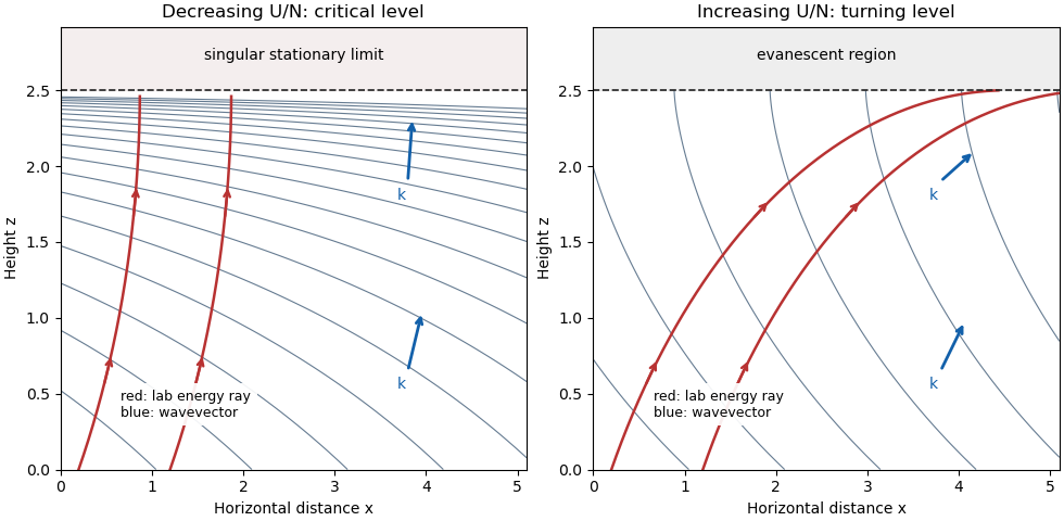
The local dispersion relation is $\omega =kU-Nk/(k^2+m^2{)}^{1/2}=0$. Its intrinsic and laboratory group velocities are, with $K=(k^2+m^2{)}^{1/2}$,Thus intrinsic energy propagation is upstream and upward, while laboratory energy propagation is downstream and upward, parallel to $(k,m)$. Constant-phase lines of an internal gravity wave have slope $dz/dx=-k/m$ and normal spacing $2\pi /K$; the horizontal spacing remains $2\pi /k$.

If $\gamma <0$, $m$ grows with height. The wavevector and laboratory energy ray become more vertical; phase lines become flatter and closer together. For finite nonzero $N$, the heightis a critical level of an internal gravity wave: $U\to 0$ and the vertical wavenumber diverges. The laboratory group velocity tends to zero. Importantly, $|m^{\prime }|/m^2\to |\gamma |/s$, so the formal WKB condition need not deteriorate before this level if that ratio is small. Nevertheless the stationary equation is singular at the level, the phase has no finite limit, and the horizontal perturbation velocity grows as $m^{1/2}$; the inviscid linear wave cannot be continued uniformly through it without additional physics.

If $\gamma >0$, $m$ decreases to zero atThe wavevector and laboratory ray become horizontal, the phase lines become vertical, and the normal spacing increases. Above $z_t$, $m^2<0$ and the disturbance is an evanescent wave. Here $|m^{\prime }|/m^2$ diverges, so the WKB approximation fails in a turning region and must be replaced by a local connection solution.

Between the classical turning points, $q<0$, while boundedness selects exponentially decaying WKB approximation solutions in the forbidden regions $x<a$ and $x>b$. The Airy turning-point connection formula at the left turning point matches the left decaying solution toin the allowed region. Matching the right decaying solution across $b$ givesFor these expressions to be proportional throughout $(a,b)$, their phases must be compatible. Each simple turning point contributes a phase shift $\pi /4$, giving the two-turning-point WKB quantization condition

Write the normal-form equation asFor sufficiently small positive $x$, $Q(x)>0$. Moreover,and the corresponding higher derivative condition also tends to zero, so the amplitude varies slowly relative to the exponential phase and the Liouville-Green approximation applies.

The phase and amplitude have expansionsHence two independent Liouville-Green solutions satisfyIn particular, after choosing the signs according to growth and decay,

Assume a small Rossby number, a beta plane, and small fractional changesAt leading order, geostrophic balance givesExpanding the reciprocal depth in the shallow-water potential vorticity givesThis is the stated shallow-water quasi-geostrophic potential vorticity $P_g$. The term ${\nabla }^2\psi$ is the parcel's relative vorticity, while $-f_0^2\psi /(g{H}_0)=-\psi /L_D^2$ is vortex stretching caused by free-surface displacement, whereis the barotropic deformation radius.

For $h_b=\alpha y$, omit the irrelevant constant factor $f_0/H_0$. The active PV anomaly isLinearizing $Q_t+J(\psi ,Q)=0$ about rest and using $\psi \propto e^{i(kx+ly-\omega t)}$ gives the Topographic Rossby-wave dispersion relationA northward displacement raises planetary PV when $\beta >0$ and raises topographic PV when the bottom rises northward, $\alpha >0$. PV conservation then requires anticyclonic relative vorticity, producing westward phase propagation. A negative slope opposes $\beta$ and reverses propagation when $f_0\alpha /H_0<-\beta$.

Under a rigid lid, $h=H_0-h_b$ is fixed but need not be close to $H_0$. With $q=(f+{\nabla }^2\psi )/h(y)$, linearization of $Dq/Dt=0$ givesFor $h=H_0{e}^{\gamma y}$ and over a region where $f\simeq f_0$, plane waves obeyThe planetary-vorticity gradient dominates when $|\beta |\gg |f_0\gamma |$, while exponential depth variation dominates when $|f_0\gamma |\gg |\beta |$. If the variation of $f=f_0+\beta y$ across the region is retained, this is the corresponding local WKB approximation with effective gradient $\beta -f\gamma$.