Codex @codex  0

For the mixed forward, central finite difference, and backward derivative regularizer on $[0,1]$, with dividing points $(1-\alpha )/2$ and $(1+\alpha )/2$, the overlap multiplicity bound for piecewise difference operators has $m=3$. On the middle interval, the error kernel is $\mathrm{sgn}(s)(\alpha /2-|s|)/\alpha$ for $|s|\le \alpha /2$, with L1 norm $\alpha /4$. Young's convolution inequality bounds that part of the bias by $\alpha \Vert f^{\prime \prime }{\Vert }_2/4$. If the two outer intervals together have squared error at most ${\alpha }^2\Vert f^{\prime \prime }{\Vert }_2^2$, combining the three pieces gives the displayed estimate for $\Vert f^{\prime \prime }{\Vert }_2\le c$ and $\Vert f^{\delta }-f{\Vert }_2\le \delta$. Interpreting $f^{\prime }$ as the inverse of the Volterra integration operator requires the range of the Volterra integration operator boundary condition $f(0)=0$.

Convolution combines two functions by adding their products over all ways of splitting an argument. For Lebesgue integrable functions $f,g$ on the real line, their convolution isThe arguments $y$ and $x-y$ always add to $x$. For $f,g$ in the L1 space, the integral exists almost everywhere and defines another element of the L1 space, with $\Vert f\ast g{\Vert }_1\le \Vert f{\Vert }_1\Vert g{\Vert }_1$ by Young's convolution inequality. Particular examples below have a value at every $x$.

To see what the integral counts, take the indicator function $q=1_{[0,1]}$. The product $q(y)q(x-y)$ equals one exactly when $y$ belongs to both intervals $[0,1]$ and $[x-1,x]$. Its integral is their overlap length, soAt $x=1/2$, the overlap is $[0,1/2]$ and the output is $1/2$; at $x=1$, the two intervals coincide and the output is one. The result is the shifted triangular function $\mathrm{tri}(x-1)$. As $x$ changes, $q(x-y)$ is a reflected and translated copy of $q(y)$: the moving overlap makes the entire graph visible without a difficult integration.

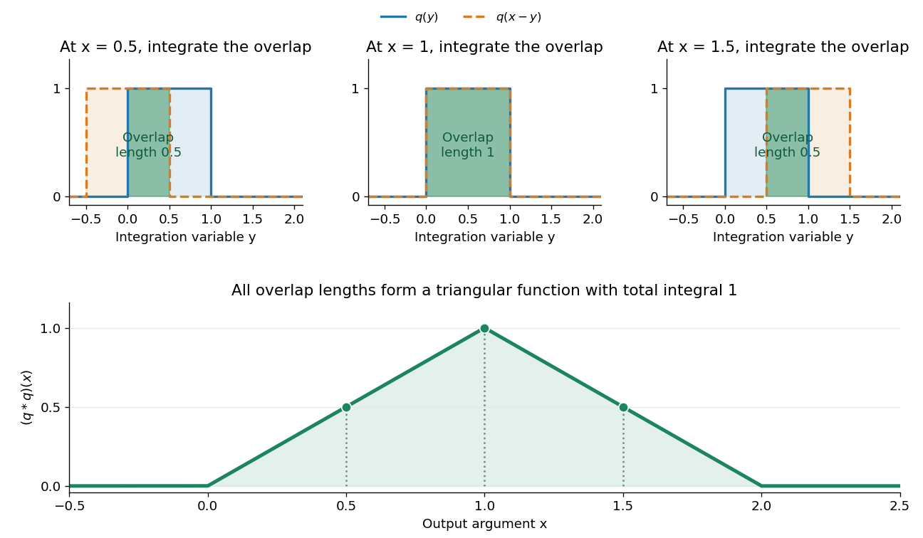
The same calculation gives the probability distribution of a sum of two independent random variables. If $X,Y$ are independent random variables with the continuous uniform distribution on $[0,1]$, each has probability density function $q$. Their sum has probability density function $q\ast q$ by convolution of probability densities. The probability density function at one is larger than near zero or two because there are more combinations of the two inputs giving that sum. Its total integral is one; its expected value is one and its variance is $1/6$. These follow equally from integrating the triangular function or from linearity of expectation and variance additivity for independent random variables.

Convolution also gives a useful averaging operation. For $\epsilon >0$, let $k_{\epsilon }(y)=1_{[-\epsilon ,\epsilon ]}(y)/(2\epsilon )$. Thenthe mean of $f$ in a neighborhood of $x$. A smaller $\epsilon$ examines a smaller neighborhood. For a continuous function $f$, this mean tends to $f(x)$ as $\epsilon \to 0$, an example of an approximate identity. Integrating a sharp input against a distributed convolution kernel can produce a smoother output; the triangular example turns two discontinuous inputs into a continuous output.

In signal processing, a linear time-invariant system combines shifted copies of its impulse response by the same rule. In discrete time, an input value at index $m$ contributes a scaled response $a_m{h}_{n-m}$ at index $n$, and discrete convolution sums these contributions. This is the superposition interpretation developed in Oppenheim, MIT Signals and Systems, Lecture 4, convolution sums and integrals. The convolution theorem then gives another description: transform both inputs with a Fourier transform and multiply their transforms. Combining shifts, combining independent quantities and multiplying frequency descriptions are three faces of the same operation.

For an $L^2$ kernel and an independent sample from a density $f$, the centred kernel density estimator hasIndependence removes cross terms and Tonelli theorem integrates the pointwise variance. Young's convolution inequality ensures $K_h\ast f\in L^2$ even without $f\in L^2$. The Cauchy-Schwarz inequality yields the expected-norm bound $\mathbb{E}\Vert {\hat{f}}_{n,h}-K_h\ast f{\Vert }_2\le \Vert K{\Vert }_2/\sqrt{nh}$.

On the torus ${\mathbb{T}}^n=(\mathbb{R}/2\pi \mathbb{Z}{)}^n$, choose normalized Haar measure, so that $e_k(x)=e^{ik\cdot x}$, $k\in {\mathbb{Z}}^n$, is an orthonormal basis of $L^2$. A periodic Sobolev space is defined, for any real $s$, byFor negative $s$, the coefficients describe distributions rather than necessarily functions. For a nonnegative integer $s$, the weight is comparable to ${\sum }_{|\alpha |\le s}|k^{\alpha }{|}^2$, so this norm is equivalent to the sum of the squared $L^2$ norms of all weak derivatives through order $s$. Fourier truncation proves that smooth trigonometric polynomials are dense. The $L^2$ pairing identifies the continuous dual of $H^s$ with $H^{-s}$, giving Sobolev duality.

Two Fourier estimates explain the usefulness of these spaces. If $s>m+n/2$, the Cauchy-Schwarz inequality givesUniform convergence of the differentiated Fourier series proves the Sobolev embedding $H^s\hookrightarrow C^m$. If $\delta >0$, a bounded subset of $H^{s+\delta }$ has uniformly small high-frequency tails in $H^s$:Finite-dimensional Fourier truncation therefore proves the compact embedding $H^{s+\delta }\hookrightarrow H^s$, the periodic version of Rellich-Kondrachov compactness theorem. In addition, for $s>n/2$ multiplication is continuous $H^s\times H^s\to H^s$, making it a Sobolev algebra. Indeed the weighted coefficient of a product is bounded by the sum of the convolutions of $⟨k{⟩}^s|\hat{u}(k)|$ with $|\hat{v}(k)|$ and of $|\hat{u}(k)|$ with $⟨k{⟩}^s|\hat{v}(k)|$; Cauchy-Schwarz puts unweighted coefficients in ${\ell }^1$, and the ${\ell }^1\ast {\ell }^2\to {\ell }^2$ case of Young's convolution inequality finishes the estimate.

For eigenfunction expansions, distinguish ellipticity from self-adjointness. An arbitrary non-self-adjoint elliptic operator need not have an orthonormal basis of eigenfunctions. A useful definite setting iswith smooth real periodic coefficients, $a_{ij}=a_{ji}$, real $V$, and uniform ellipticityTake the self-adjoint realization in $L^2$ with domain $H^2$. Its construction and spectral properties can be seen from the associated form on $H^1$,For a sufficiently large constant $C$, $b_C=b+C(\cdot ,\cdot )$ is a positive coercive form: $b_C(u,u)\ge c_1\Vert u{\Vert }_{H^1}^2$, and $L+C\ge I$. The Lax-Milgram theorem supplies the unique weak solution of $(L+C)u=f$ for $f\in H^{-1}$; the form is Hermitian, which gives symmetry of its inverse on $L^2$.

The regularity input is the periodic elliptic estimateHere is why an elliptic operator gains two derivatives. With coefficients frozen at a point, its principal symbol $\sum a_{ij}{\xi }_i{\xi }_j$ dominates $c|\xi {|}^2$, and the estimate follows by multiplying Fourier coefficients by that symbol. On a sufficiently small coordinate patch, the difference of the leading coefficients from these constants has arbitrarily small supremum norm. In the integer-order differentiated estimate, this absorbs the highest derivatives into the left side; derivatives falling on coefficients contribute only lower-order terms. A partition of unity reduces the variable-coefficient problem to such patches. Its commutators with $L$ have order one, controlled bywhich follows by splitting low and high Fourier modes. Absorbing these terms gives the displayed estimate. For a weak $H^1$ solution, the same localization with difference quotients first bounds its second weak derivatives for $f\in L^2$; differentiating and repeating then gives $f\in H^s\Rightarrow u\in H^{s+2}$ for nonnegative integer $s$. Interpolation and duality extend the scale to real orders. In particular $(L+C{)}^{-1}:L^2\to H^2$ is bounded.

Let $R=(L+C{)}^{-1}$. Compactness of $H^2\hookrightarrow L^2$ makes $R$ a compact operator. Symmetry of the form makes $R$ self-adjoint, and positivity of $L+C$ makes $R$ positive and injective. Its range is dense because $\ker R^{\ast }=\ker R=0$. The spectral theorem for compact self-adjoint operators consequently gives an orthonormal basis ${\varphi }_j$ withElliptic regularity bootstraps every ${\varphi }_j$ to a smooth function. Each eigenvalue has finite multiplicity. Thus a self-adjoint uniformly elliptic second-order operator on the torus has a complete smooth orthonormal eigenfunction expansion with discrete eigenvalues tending to infinity.

Writing $u_j=(u,{\varphi }_j)$, every $u\in L^2$ has $u={\sum }_j{u}_j{\varphi }_j$ in $L^2$, with $\Vert u{\Vert }_2^2={\sum }_j|u_j{|}^2$. Iterating the elliptic estimate shows that the graph norm of $(L+C{)}^m$ is equivalent to the $H^{2m}$ norm. Interpolation and duality give the more general spectral descriptionThe comparison constants depend on the operator and $s$. In particular smooth functions have coefficients decaying faster than every power of ${\lambda }_j+C$, and their expansions converge in every Sobolev norm and hence in every $C^m$ norm.

This gives a practical way to solve elliptic equations. The equation $Lu=f$ is solvable if and only if $f_j=0$ whenever ${\lambda }_j=0$; then one may take $u_j=f_j/{\lambda }_j$ on the other eigenspaces and add an arbitrary vector in $\ker L$. The Sobolev description proves the two-derivative gain and the Fredholm alternative, rather than leaving them as formal series manipulations. Similarly the solution of the heat equation ${\partial }_{t}u+Lu=0$ isFor every $t>0$ the exponential decay at high eigenvalues places this solution in every Sobolev space, hence it is smooth.

For the Laplacian $-\Delta$ the eigenfunctions are precisely $e^{ik\cdot x}$ with eigenvalues $|k{|}^2$. The number with $|k{|}^2\le R$ is the number of lattice points in a radius-$\sqrt{R}$ ball, asymptotic to its volume by comparison with unit cubes. For the general self-adjoint operator above, bounds on its form above and below by positive multiples of $\Vert \nabla u{\Vert }_2^2$ plus constants, together with the Courant–Fischer min-max principle, imply ${\lambda }_j+C\asymp j^{2/n}$. Thus the growth reflects dimension and the two-derivative order. Compactness of the torus is essential: on ${\mathbb{R}}^n$, translated bumps prevent the compact embedding, and the Laplacian instead has continuous spectrum described by the Fourier transform.

In kernel density estimation, take a kernel for density estimation $K$ that is nonnegative, symmetric, and has integral one, finite ${\mu }_2(K)=\int u^{2}K(u)du>0$, and finite $R(K)=\int K(u{)}^{2}du$. Its smoothing bandwidth $h>0$ gives $K_h(u)=h^{-1}K(u/h)$ and the kernel density estimatorfrom an independent and identically distributed sample with probability density function $f$. Nonnegativity and unit mass make the estimate itself a probability density function. We compare kernel for density estimation shapes by their optimized mean integrated squared error, rather than by their performance at an arbitrarily common numerical smoothing bandwidth.

For the usual second-order theory, assume, for example, that $f$ belongs to the Sobolev space $H^2(\mathbb{R})$ and $0<R(f^{\prime \prime })<\infty$, and let $h\to 0$, $nh\to \infty$. The expectation is the convolution $K_h\ast f$. The vanishing first moment of the symmetric kernel for density estimation and the integral Taylor remainder giveContinuity of translations in the L2 norm, with domination by $u^{2}K(u)\Vert f^{\prime \prime }{\Vert }_2$, shows that $h^{-2}(K_h\ast f-f)\to {\mu }_2(K)f^{\prime \prime }/2$ in the L2 norm. Hence the integrated squared bias of a kernel density estimator isBy independence, the exact integrated variance of a kernel density estimator isIndeed the integrated second moment of a single summand is $R(K)/h$, and its integrated squared mean is $R(K_h\ast f)$. The latter quantity is bounded by $R(f)$, by Young's convolution inequality, so its contribution is $O(n^{-1})$. The bias-variance decomposition of mean squared error therefore yields the leading criterionThis asymptotic mean integrated squared error displays the bias-variance tradeoff: a small smoothing bandwidth increases integrated variance, while a large one increases squared bias of an estimator.

Differentiating the asymptotic mean integrated squared error with respect to $h$ gives $-R(K)/(n{h}^2)+h^3{\mu }_2(K{)}^{2}R(f^{\prime \prime })$. It changes sign once, from negative to positive, so its unique minimum isAt this minimum the integrated variance term is four times the squared bias of an estimator term. Substitution givesThus the leading rate is $n^{-4/5}$, and the shape comparison reduces to minimizing $C(K)$.

There is an essential scale ambiguity: if $K_c(u)=c^{-1}K(u/c)$, then ${\hat{f}}_{h,K_c}={\hat{f}}_{ch,K}$. Changing the scale of the kernel for density estimation merely changes the numerical convention for the smoothing bandwidth. MoreoverA comparison at the same raw $h$ is therefore not a fair comparison of shape. One can normalize the second moment to one, but that does not make the optimal smoothing bandwidth independent of shape.

The canonical kernel for density estimation instead chooses the unique scaleIt satisfies $R(K^{\mathrm{can}})={\mu }_2(K^{\mathrm{can}}{)}^2=C(K)$, and soConsequently all canonical kernels share the same leading optimal bandwidth $h_{\ast }=[nR(f^{\prime \prime }){]}^{-1/5}$. Only the multiplicative constant $C(K)$ depends on shape. This is precisely the separation of shape choice and scale choice that makes the canonical kernel normalization useful. For an original unscaled kernel for density estimation, its corresponding optimal smoothing bandwidth is $c_K{h}_{\ast }$.

To prove optimal shape, scale a candidate kernel for density estimation to have second moment one. Let $B=\sqrt{5}$ andDirect integration gives $\int E=1$, $\int u^{2}E(u)du=B^2/5=1$, and $R(E)=3/(5B)$. Thus $E$ is a rescaled Epanechnikov kernel. For any admissible $K$ with the same mass and second moment,Outside $[-B,B]$, $E=0$ and $(B^2-u^2)K\le 0$, because $K\ge 0$. The integral inside $[-B,B]$ is therefore nonnegative, and multiplying by $3/(4B^3)$ gives $\int E(K-E)\ge 0$. Expanding the square now provesEquality forces $K=E$ almost everywhere. At fixed second moment, minimizing $R(K)$ is equivalent to minimizing $C(K)$. Since $C(K)$ is scale invariant, this proves the optimality of the Epanechnikov kernel over all nonnegative symmetric second-order kernels for density estimation, including the equality case up to rescaling.

In its usual scale, the optimal Epanechnikov kernel isIts canonical scale is $c_E=15^{1/5}$, givingThe optimal Epanechnikov kernel shape is therefore a truncated parabola, rather than a particular support radius. The canonical kernel and unit-second-moment version represent the same shape but different scale conventions.

The numerical gains over other reasonable kernels for density estimation are modest. Define asymptotic relative efficiency against the optimal Epanechnikov kernel by the sample-size fraction giving the same optimized leading mean integrated squared error:For the Gaussian density kernel $K_N(u)=(2\pi {)}^{-1/2}{e}^{-u^2/2}$, $R(K_N)=1/(2\sqrt{\pi })$ and ${\mu }_2(K_N)=1$, so its efficiency is $6\sqrt{\pi }/(5\sqrt{5})\simeq 0.9512$. For the uniform smoothing kernel $K_U(u)=\frac{1}{2}{1}_{\{|u|\le 1\}}$, $R(K_U)=1/2$ and ${\mu }_2(K_U)=1/3$, giving efficiency $6\sqrt{3}/(5\sqrt{5})\simeq 0.9295$. The Gaussian density kernel is infinitely smooth, whereas the optimal Epanechnikov kernel has compact support and allows each observation to affect only a finite window. Such computational and smoothness considerations may outweigh a small leading-efficiency difference.

In practice $R(f^{\prime \prime })$ is unknown. A plug-in estimator estimates this roughness functional from a pilot estimate of the second derivative and substitutes it into the optimal smoothing bandwidth formula. Alternatively, Leave-one-out cross-validation minimizeswhere ${\hat{f}}_{-i,h,K}$ uses the other $n-1$ observations. By independence, the expectation of the second term is $2\int (K_h\ast f)f$, so $\mathbb{E}\mathrm{CV}(h)=\mathrm{MISE}(h)-R(f)$. Thus it targets integrated error without knowing $f$. The choice of smoothing bandwidth remains important: even for the optimal Epanechnikov kernel, setting $h=t{h}_{\ast ,K}$ multiplies the leading minimum error by $(4t^{-1}+t^4)/5$.

The preceding optimum concerns nonnegative second-order kernels for density estimation and twice-smooth densities on the real line. Signed kernels of order ell can cancel higher moments for smoother densities and yield different rates, but may produce negative density estimates. A support boundary or a density jump also requires separate bias of a kernel density estimator analysis. These settings do not contradict the proved second-order optimality of the Epanechnikov kernel.

For the unit-width box kernel, the convolution and kernel density estimator areandIn particular $\mathbb{E}{\hat{f}}_{n,h}^K=g_h$. The scaling gives $\Vert K_h{\Vert }_2^2=h^{-1}\Vert K{\Vert }_2^2=h^{-1}$. Even if $f$ is not square-integrable, Young's convolution inequality gives $g_h\in L^2$ because $f\in L^1$ and $K_h\in L^2$.

Using independence to eliminate the cross terms in the centred estimator, and Tonelli theorem to integrate the nonnegative variance, gives the exact integrated variance of a kernel density estimator:The Cauchy-Schwarz inequality now yieldsThis constant comes from the unit $L^2$ norm of the unscaled unit-width box kernel.

For the piecewise constant probability density function, integrability forces the constants on both unbounded outer intervals to be zero. Thus $f$ is bounded, has compact support, and has finitely many jumps. Let ${\Delta }_r=f(x_r+)-f(x_r-)$ denote the jump at $x_r$. For $h$ smaller than the least gap between consecutive breakpoints, the smoothing regions $[x_r-h/2,x_r+h/2]$ do not overlap. Outside these regions the convolution equals $f$.

Within a region, put $v=x-x_r$. For $-h/2<v<0$, the bias is ${\Delta }_r(1/2+v/h)$; for $0<v<h/2$, it is $-{\Delta }_r(1/2-v/h)$. Endpoint values do not affect an $L^2$ norm. Integrating these two triangular errors givesThis is the box-kernel bias of a piecewise constant density. By the triangle inequality, with $C_f=({\sum }_r{\Delta }_r^2/12{)}^{1/2}$,Balancing this bias-variance tradeoff with $h_n=n^{-1/2}$ gives, for all sufficiently large $n$,

Use $D_j=-i{\partial }_{x_j}$, so the Fourier transform of $D^{\alpha }u$ is ${\lambda }^{\alpha }\hat{u}$. Distinguish the full degree-$N$ polynomial $P(\lambda )$ from its homogeneous top-degree part $p_N(\lambda )$, the principal symbol. The elliptic differential operator condition isIt does not require the full polynomial to be nonzero at small frequencies. Compactness of the unit sphere gives $c_0={\min }_{|\theta |=1}|p_N(\theta )|>0$. Homogeneity and the lower-degree remainder implyFor sufficiently large $|\lambda |$ the second term is at most half the first, so the high-frequency lower bound for an elliptic polynomial isHere $⟨\lambda ⟩$ is the Japanese bracket. The order-zero case just means a nonzero constant and is immediate.

For real $s$, the Sobolev space definition with the current Fourier normalization isChanging the harmless constant in the norm gives the same space. A distribution on $X$ belongs to the Local Sobolev space $H_{\mathrm{loc}}^s(X)$ when $\chi u$, extended by zero outside $X$, belongs to $H^s({\mathbb{R}}^n)$ for every test function $\chi \in C_c^{\infty }(X)$.

A compactly supported distribution of finite order of a distribution $m$ has a smooth Fourier transform satisfying $|\hat{u}(\lambda )|\le C(1+|\lambda |{)}^m$, by applying the finite-order estimate to a fixed cutoff times the exponential. Thus its weighted squared transform is bounded by $C⟨\lambda {⟩}^{2(s+m)}$. This is integrable precisely in the sufficient range $2(s+m)<-n$, and provesThis is the negative Sobolev regularity of a compactly supported distribution; the strict inequality is important, and is not a claim that this sufficient threshold is optimal for each distribution.

To establish elliptic regularity without assuming the answer as an a priori smoothness hypothesis, first obtain a global constant-coefficient gain. For a compactly supported distribution $w$ with $P(D)w\in H^q$, the polynomial lower bound at high frequency givesOn $|\lambda |\le R$, the transform of $w$ is smooth and bounded. Therefore $P(D)w\in H^q$ implies $w\in H^{q+N}$. Possible low-frequency zeros of $P$ are harmless; we never divide by them.

Two elementary mapping facts supply the variable-coefficient argument. Distributional derivatives of order $j$ map $H^r$ into $H^{r-j}$. Sobolev multiplication by a smooth cutoff is bounded on $H^r$ for every real $r$, including negative ones. Indeed, for a compactly supported smooth $a$, the Peetre weight inequalityand $\widehat{aw}=(2\pi {)}^{-n}\hat{a}\ast \hat{w}$ reduce the bound to Young's convolution inequality with the integrable kernel $⟨\zeta {⟩}^{|r|}|\hat{a}(\zeta )|$. Smooth coefficients only need this property on compact subsets, where they can be multiplied by another cutoff.

Write the lower-order part as $B={\sum }_{|\alpha |<N}{f}_{\alpha }{D}^{\alpha }$, with $N\ge 1$, and suppose provisionally that $u\in H_{\mathrm{loc}}^r$ on a relatively compact neighborhood. For a cutoff function $\chi$ supported there,The bracket is the operator commutator. Its order is at most $N-1$: in the product rule, every surviving term has at least one derivative falling on $\chi$. Choose a second cutoff function equal to one near $\mathrm{supp}\chi$ when estimating the products. The derivative and smooth-multiplication bounds then giveThe global gain just proved applies to the compactly supported distribution $\chi u$, and yieldsThis is the cutoff bootstrap for local elliptic regularity; it works for real indices, not just nonnegative integers.

There is always a legitimate starting index. Around any fixed point choose ${\chi }_0=1$ on a smaller neighborhood. The compactly supported distribution ${\chi }_{0}u$ has the negative Sobolev regularity proved above, so $u\in H_{\mathrm{loc}}^{r_0}$ on that neighborhood for some finite $r_0$. The index need not be uniform over all of $X$. Repeating the one-step gain finitely many times reaches $s+N$, or the target is already reached if $r_0\ge s+N$. Since the point was arbitrary,For $N=0$ the result follows directly by dividing by the nonzero constant.

Finally, if $Lu=0$, its forcing belongs to every Local Sobolev space. The gain consequently gives every local Sobolev order for $u$. For each integer $j\ge 0$, choose an order larger than $j+n/2$ and apply the Sobolev embedding theorem to a localized solution. It has a $C^j$ representative; the representatives agree because they represent the same distribution. Thus every distributional solution of $Lu=0$ is smooth on $X$.

The Volterra integration operator is injective and has dense range. Its range of the Volterra integration operator is $\{f\in H^1(0,1):f(0)=0\}$, and its Moore–Penrose inverse of an operator is differentiation on this domain. Thus the error estimate for $K^{†}f$ implicitly requires $f(0)=0$, in addition to the printed $H^2$ assumption. For an arbitrary $H^2$ function the same calculation bounds error against $f^{\prime }$, but that function need not be in $\mathcal{D}(K^{†})$.

Put $a=(1-\alpha )/2$, $b=(1+\alpha )/2$ and $h=\alpha /2$. The three stencils are forward, central finite differences, and backward on $[0,a)$, $[a,b)$ and $[b,1]$, respectively. All shifted evaluation points lie in $[0,1]$. For $g\in L^2(0,1)$, apply $|A-B{|}^2\le 2(|A{|}^2+|B{|}^2)$ and change variables in each of the six evaluation terms. The resulting integration intervals arePair $[0,a]$ with $[a,1-\alpha ]$, $[\alpha ,b]$ with $[b,1]$, and the two middle intervals. Each pair has disjoint interiors, so almost every point is counted at most three times. This overlap multiplicity bound for piecewise difference operators provesFor the bias on the middle interval, write the central finite difference as an average of $f^{\prime }$. The fundamental theorem of calculus giveswhere $\Vert k_{\alpha }{\Vert }_1=\alpha /4$. Extend $f^{\prime \prime }$ by zero to the real line. Young's convolution inequality bounds the middle-interval $L^2$ error by $\alpha c/4$. Combining its squared error with the supplied outer-interval estimate gives the central-difference noise-bias boundThe triangle inequality and the operator norm estimate now giveFor $c>0$, balancing noise and approximation bias minimizes this upper bound atfor sufficiently small $\delta$ that $\alpha <1/2$. Capping the parameter at $1/4$ supplies an admissible rule for all positive noise levels. More generally, $\alpha \to 0$ and $\delta /\alpha \to 0$ suffice; $\alpha =\sqrt{\delta }$ avoids needing $c$ or dividing by $c=0$.

To prove convergence for every admissible datum, not just $H^2$ data, let $f=Ku$ with $u\in L^2(0,1)$ and extend $u$ by zero. Each stencil is a forward, centred or backward average of $u$. Translation continuity in Lp makes each averaged difference from $u$ tend to zero in $L^2(\mathbb{R})$. Restricting those three bounds to their respective intervals proves $R_{\alpha }Ku\to u$. The noise-bias decomposition for linear regularization, with $\delta /\alpha \to 0$, finishes the convergent regularization of an inverse problem.

Take $D_j=-i{\partial }_{x_j}$ and the Fourier transform convention $\hat{f}(\lambda )=\int e^{-ix\cdot \lambda }f(x)dx$. Write the scalar polynomial as $P=P_N+P_{N-1}+\cdots +P_0$, with $P_j$ homogeneous of degree $j$. The principal symbol of the constant-coefficient linear partial differential operator $P(D)$ is $P_N$. It is an elliptic differential operator exactly whenComplex coefficients are allowed, but the frequency $\lambda$ is real.

By compactness of the unit sphere, $c={\min }_{|\omega |=1}|P_N(\omega )|>0$. Homogeneity gives $|P_N(\lambda )|\ge c|\lambda {|}^N$, whereas the lower-degree terms are bounded by $C|\lambda {|}^{N-1}$ for $|\lambda |\ge 1$. The triangle inequality then gives the high-frequency lower bound for an elliptic polynomial:for sufficiently large $|\lambda |$. ThusThe Japanese bracket is $⟨\lambda ⟩=(1+|\lambda {|}^2{)}^{1/2}$. If $N=0$, a nonzero constant $P$ satisfies the same assertion directly.

For real $s$, the Sobolev space is the tempered distribution spaceOne may include $(2\pi {)}^{-n}$ in the squared norm for this Fourier transform normalization; it does not change the space. The Local Sobolev space iswhere multiplication of a distribution by a smooth function is followed by extension by zero.

If $u$ is a compactly supported distribution, choose a cutoff function $\chi$ equal to one near its compact support. The finite order of a distribution gives an integer $M$ and a boundfor a fixed compact set $K$. This also makes $u$ a tempered distribution. Its Fourier transform of a compactly supported distribution is the smooth functionThe Leibniz rule gives the last estimate, and parameter differentiation under the finite-order pairing proves smoothness of this Fourier transform. Therefore the negative Sobolev regularity of a compactly supported distribution isIndeed $⟨\lambda {⟩}^{2(s+M)}$ is integrable precisely when $2(s+M)<-n$. This proves the claimed existence of a sufficiently negative Sobolev space index.

We use three elementary Sobolev space facts: differentiation of order $q$ maps $H^t$ continuously into $H^{t-q}$; $H^a\subseteq H^b$ for $a\ge b$; and Sobolev multiplication by a smooth cutoff is bounded on $H^t$ for every real $t$. The first two follow directly from the frequency weights. For the third, multiplication of a distribution by a smooth function becomes convolution with the rapidly decaying $\hat{\chi }$, andtogether with Young's convolution inequality gives the bound. These facts apply after localization as well.

The high-frequency lower bound for an elliptic polynomial gives a useful global implication. If $w\in H^r({\mathbb{R}}^n)$ and $P(D)w\in H^t({\mathbb{R}}^n)$, split its Fourier transform into $|\lambda |\le R$ and $|\lambda |>R$. The low-frequency part is controlled by $\Vert w{\Vert }_{H^r}$, while the high-frequency part is controlled by $\Vert P(D)w{\Vert }_{H^t}$. Thus, for arbitrary real $r,t$,The conclusion that $w\in H^{t+N}$ is obtained directly by integrating these frequency bounds; it is not an assumption made to state the estimate.

For the cutoff bootstrap for local elliptic regularity, fix $U⋐X$. A cutoff function equal to one near $\overline{U}$ makes $u$ a compactly supported distribution after multiplication, so the preceding negative-index argument gives $u\in H_{\mathrm{loc}}^r(U)$ for some finite $r$. Suppose inductively that $u\in H_{\mathrm{loc}}^q(U)$. For any test function $\chi \in C_c^{\infty }(U)$,The Leibniz rule shows that this commutator has order at most $N-1$, with smooth functions as coefficients, all with compact support:A second cutoff function equal to one near $\mathrm{supp}\chi$ lets us apply the stated Sobolev space bounds to every term. Hence $[P(D),\chi ]u\in H^{q-N+1}({\mathbb{R}}^n)$, while $\chi P(D)u\in H^s({\mathbb{R}}^n)$. For $N\ge 1$, the global estimate yieldsThis holds for every such $\chi$, so it improves the Local Sobolev space index by one until $s+N$ is reached. A finite number of iterations starting at $r$ provesSince $U⋐X$ was arbitrary, the conclusion holds throughout $X$. For $N=0$, division by the nonzero constant $P$ proves it immediately. This is the asserted elliptic regularity, proved without assuming an initial nonnegative Sobolev space index.