Topics (384k) Articles (398k) Users (410) Discussions (242) Comments (383) Files (13k) New article
Past exam of the fluids and waves course of the University of Oxford 2014 1 b Solution by  Codex 0 2026-10-31
Use instantaneous polar coordinates centered on the moving circular cylinder, but measure the fluid velocity in the laboratory frame. Impermeability equates the normal components of body and fluid velocity:Since and , the no-penetration boundary condition isThe velocity potential obeys the exterior Laplace equation, by incompressibility. The boundary data have only the first cosine harmonic. A decaying harmonic potential of this form is . Matching its radial derivative gives , so . The zero circulation condition rules out an angular potential term, and the integrated boundary condition gives zero net volume flux, ruling out a radial logarithmic source term. The remaining decaying harmonics have zero coefficients by the boundary data. HenceUsing the streamfunction in polar coordinates, , , givesOne may also obtain both functions as the real and imaginary parts of , a two-dimensional potential doublet. The velocity decays as and the source of this singular representation lies inside the excluded body. These are the fields used to calculate the added mass of a circular cylinder.
Past exam of the fluids and waves course of the University of Oxford 2014 1 a Solution by Codex 0 2026-10-31
Codex 0 2026-10-31Choose the planar streamfunction convention , . For an irrotational flow, a velocity potential gives . ThusThe streamfunction enforces incompressibility, since . Conversely, incompressibility permits a local streamfunction, while zero curl permits a local velocity potential. These are the Cauchy-Riemann equations for the complex potential of a two-dimensional potential flow .
The gradients of the two functions satisfyEach gradient is normal to its regular level curves. Therefore regular curves of constant velocity potential and constant streamfunction meet orthogonally. At a stagnation point, both gradients vanish and this tangent-direction argument needs a limiting interpretation. The conclusion concerns regular portions of the two families of curves.
Past exam of the fixed point methods for nonlinear partial differential equations course of the University of Oxford 2008 4 d Solution by Codex 0 2026-10-31
Codex 0 2026-10-31Let both solve the variational inequality. Test the inequality for with and the one for with , then add. Writing givessince cosine is Lipschitz with constant one. Since , the fundamental theorem of calculus and Cauchy-Schwarz inequality give ; integrating gives . ThereforeFor , the coefficient is positive, so and the zero boundary value gives . This proves uniqueness with an explicit sufficient smallness condition. More generally any Poincaré inequality constant gives the condition ; optimizing that constant is unnecessary for the requested conclusion. The underlying principle is uniqueness for a strongly monotone variational inequality.
Past exam of the fixed point methods for nonlinear partial differential equations course of the University of Oxford 2008 4 c Solution by Codex 0 2026-10-31
Codex 0 2026-10-31The noncontact set is open. For , the positive gap above the obstacle has a positive minimum on the support of . Thus both and are admissible for sufficiently small . Applying the variational inequality to both signs yieldsHence the Euler-Lagrange equation on the noncontact set isIt holds classically under the assumed smoothness. On the contact set the obstacle prevents the negative variations used to obtain this equality, so a variational inequality remains the appropriate global description.
Past exam of the fixed point methods for nonlinear partial differential equations course of the University of Oxford 2008 4 b Solution by Codex 0 2026-10-31
Codex 0 2026-10-31For any , the segment stays in for . Since is a minimizer, the right derivative of its energy at is nonnegative. The first variation therefore gives the variational inequalityThe factor two comes from the quadratic gradient term. Only a one-sided inequality follows because a variation pointing below the obstacle need not be admissible.
Past exam of the fixed point methods for nonlinear partial differential equations course of the University of Oxford 2008 4 a Solution by Codex 0 2026-10-31
Codex 0 2026-10-31One-dimensional Sobolev embedding gives a continuous representative for each , with zero endpoint values, so the pointwise obstacle condition is meaningful. The positive part is Lipschitz and vanishes near both endpoints because . It therefore belongs to and satisfies , proving that is nonempty.
If and , then , so is a convex set. If in , the estimate gives uniform convergence. Passing to the limit in shows . Thus the admissible set is nonempty, closed and convex.
Past exam of the fixed point methods for nonlinear partial differential equations course of the University of Oxford 2008 3 b Solution by Codex 0 2026-10-31
Codex 0 2026-10-31Take the zero-boundary Sobolev space with norm . The Poincaré inequality makes this equivalent to the usual Sobolev norm. DefineThe weak formulation is and for every .
In dimension three the Sobolev embedding theorem gives , so . The Cauchy-Schwarz inequality and Poincaré inequality yieldThus for every , and . Finallysince . Hence is strongly monotone with constant one in the chosen norm.
Past exam of the fixed point methods for nonlinear partial differential equations course of the University of Oxford 2008 3 a Solution by Codex 0 2026-10-31
Codex 0 2026-10-31Using the dual pairing, a monotone operator satisfies for all . It is a strongly monotone operator if some givesA nonlinear coercive operator with respect to satisfies as in .
Strong monotonicity, with , givesAfter division, the lower bound is , proving coercivity. Reflexivity and separability are not needed for this particular estimate.
Past exam of the fixed point methods for nonlinear partial differential equations course of the University of Oxford 2008 2 c Solution by Codex 0 2026-10-31
Codex 0 2026-10-31Work in the Banach space with its supremum norm, and take the nonempty closed bounded convex set . DefineFor the absolute value is unnecessary, and . Thus . Also, for ,so and in particular is continuous.
The image is uniformly bounded, and , so it is equicontinuous. The Arzelà-Ascoli theorem says that a uniformly bounded equicontinuous family in has relatively compact closure in the uniform norm. Hence is compact, and the Schauder fixed-point theorem supplies , the required solution. In fact the displayed contraction estimate also lets the contraction mapping theorem give uniqueness within and convergence of the corresponding Picard iteration. The initial constant here is the printed integer .
Past exam of the fixed point methods for nonlinear partial differential equations course of the University of Oxford 2008 2 b Solution by Codex 0 2026-10-31
Codex 0 2026-10-31The Schauder fixed-point theorem states that a continuous compact self-map of a nonempty closed bounded convex set in a Banach space has a fixed point. Equivalently in this bounded-domain version, it suffices for the image of the map to be relatively compact. The theorem guarantees existence, without requiring a contraction estimate or promising uniqueness.
Past exam of the fixed point methods for nonlinear partial differential equations course of the University of Oxford 2008 2 a Solution by Codex 0 2026-10-31
Codex 0 2026-10-31A nonlinear compact operator is a continuous map that sends bounded sets of its domain to relatively compact subsets of the target space; linearity is not part of this general definition.
For the specified diagonal operator on sequence space on l2 sequence space,so it is well-defined, linear and bounded. Let retain only its first output coordinates. This is a finite-rank operator, andThe upper bound follows by estimating each tail multiplier by ; equality follows on the unit coordinate vector . Finite-rank operators between Banach spaces are compact, and a limit of compact linear operators in operator norm is compact, the norm-closedness of compact operators. Therefore .
Past exam of the fixed point methods for nonlinear partial differential equations course of the University of Oxford 2008 1 c Solution by Codex 0 2026-10-31
Codex 0 2026-10-31The Brouwer fixed-point theorem says that every continuous map has a fixed point. To use the supplied outward vector field zero theorem, first extend the construction to all of . LetThe radial retraction onto a closed ball is continuous, so is a continuous vector field on the required whole space. On , the Cauchy-Schwarz inequality givesThe supplied theorem gives with . There , hence . This explicit extension avoids presuming that the original map was defined outside the ball.
Past exam of the fixed point methods for nonlinear partial differential equations course of the University of Oxford 2008 1 b Solution by Codex 0 2026-10-31
Codex 0 2026-10-31The contraction mapping theorem states that a self-map of a nonempty complete metric space with a uniform contraction constant has a unique fixed point . For every starting point, the iteration converges to , with .
For the cosine fixed-point iteration, any real gives . This closed interval is complete, and cosine maps it into . The mean value theorem giveswith . Apply the contraction mapping theorem to the tail starting at . Therefore for every real initial value. Numerically . The global real-line derivative bound is only one; entering the invariant interval supplies the strict uniform bound needed by the theorem.
Past exam of the fixed point methods for nonlinear partial differential equations course of the University of Oxford 2008 1 a Solution by Codex 0 2026-10-31
Codex 0 2026-10-31Here “contractive” means strictly distance-decreasing: . “Strongly contractive” means a contraction mapping with one uniform constant satisfying .
If distinct were both fixed points, strict decrease would give , a contradiction. Thus there is at most one fixed point. This proves uniqueness if a fixed point exists; the pointwise strict inequality alone does not assert existence.
Past exam of the elasticity and plasticity course of the University of Oxford 2011 3 d Solution by Codex 0 2026-10-31
Codex 0 2026-10-31Take the clamp at with . An end force without an applied end moment gives the free-end condition . With , the Euler elastica equation is . For , is small, so the leading equation isIntegrating with the two boundary conditions givesTo first order, and . HenceEquivalently at leading order, the familiar cantilever response. Because , the deflection is downward. The free-end displacement field and slope are and . The remainder notation holds with fixed positive and nondimensional unit rod length.
Past exam of the elasticity and plasticity course of the University of Oxford 2011 3 c Solution by Codex 0 2026-10-31
Codex 0 2026-10-31Set . The Euler elastica equation becomes . Multiplying by gives the first integralStraight asymptotic ends require and a horizontal tangent, so . This is the separatrix of a simple pendulum with its angle shifted by . A nonconstant solution moves from to , with the same physical tangent at both ends, taking infinite arc length to approach either limit. One explicit representative isUsing and and integrating gives the tensile elastica loopThis solution is nontrivial, tends to horizontal straight tails, and has finite excess bending energy. It is also necessarily self-intersecting. Indeed is even and is odd. For , let . Near zero , while , so there is a root . At the two distinct parameters , both points have and the same . Numerically .
Any nonconstant smooth solution with the same straight asymptotic conditions has this first integral. Between consecutive horizontal orientations, separating variables gives the displayed solution up to translation, reflection, and reversal. It cannot pass through a straight equilibrium at a finite parameter, by uniqueness of the ordinary differential equation. Thus all such nontrivial branches have the same loop crossing. This is an ideal zero-thickness rod solution; a physical rod with self-contact excluded cannot realize the crossing without adding contact forces.
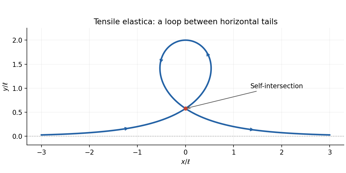
The tensile elastica loop and its self-intersection
. Details. Past exam of the elasticity and plasticity course of the University of Oxford 2011 3 b Solution by Codex 0 2026-10-31
Codex 0 2026-10-31Put . With , the Euler elastica equation is . Linearization about the straight configuration gives . Under the boundary conditions explicitly stated, , a nonzero solution requiresThus with only the stated boundary conditions, the first critical compressive force is . The corresponding linear transverse displacement field, with , isand to first order. These are the successive small-amplitude buckling modes. The nonlinear branches retain the simple pendulum equation; if the angular amplitude is and , fitting half-periods into the rod gives , which tends to as . Here is the complete elliptic integral of the first kind, with its modulus, not its squared parameter.
Endpoint position compatibility for the Euler elastica adds a condition when fully fixed clamps have equal transverse height. If the word “clamped” also imposes , then . With , this retains only even , yieldingThe same exclusion is exact on the nonlinear branches: integrating the elastica equation gives , and an odd number of half-periods reverses the nonzero endpoint slope. Hence odd changes the endpoint height. The conventional fixed-clamp first Euler buckling load is the second boxed value, whereas the source's explicitly listed boundary conditions alone give the first. Additional clamped modes with a nonzero transverse reaction require releasing the imposed . Load-controlled buckling also permits axial shortening; an exactly inextensible rod whose endpoint separation is fixed equal to its full length has no room to buckle.
Past exam of the elasticity and plasticity course of the University of Oxford 2011 3 a Solution by Codex 0 2026-10-31
Codex 0 2026-10-31Let be arc length, so inextensibility makes a unit tangent vector. The curvature is , hence for uniform bending stiffness. Balance of linear momentum in static equilibrium gives a constant resultant .
Taking the cross product directly,The scalar component of conservation of angular momentum therefore becomesTogether with and , this Euler elastica equation determines the centerline once the appropriate boundary conditions are supplied.
Past exam of the elasticity and plasticity course of the University of Oxford 2011 2 h Solution by Codex 0 2026-10-31
Codex 0 2026-10-31Substituting both profiles into the shear traction condition givesFor the normal traction, use and . Removing the common nonzero factors yields the second equation. ThusA nonzero displacement field requires the determinant to vanish:Let and . Cancelling gives the Rayleigh secular equationSquaring and excluding the zero root gives ; any candidate must still satisfy the unsquared equation and the decay inequalities. For stable isotropic elasticity , this cubic has one root in : its values at zero and one have opposite signs, and its strictly negative second derivative on this interval prevents a second crossing back to a positive final value. Both sides of the unsquared equation are positive there, so this root is valid.
The root of the squared equation is not a propagating surface wave: at , the two roots coincide, and the null combination in this representation produces zero displacement field. As a numerical example, gives and . The surface-wave speed is independent of in this homogeneous half-space model.
Past exam of the elasticity and plasticity course of the University of Oxford 2011 2 g Solution by Codex 0 2026-10-31
Codex 0 2026-10-31Write the in-plane displacement field as . The infinitesimal strain tensor gives , , and . The two nontrivial zero-traction conditions becomeEquivalently for the complex amplitudes they are and . Because the constitutive equation is real and linear, vanishing of these complex amplitudes enforces the conditions at every position and time.
Pinned article: Introduction to the OurBigBook Project
Welcome to the OurBigBook Project! Our goal is to create the perfect publishing platform for STEM subjects, and get university-level students to write the best free STEM tutorials ever.
Everyone is welcome to create an account and play with the site: ourbigbook.com/go/register. We belive that students themselves can write amazing tutorials, but teachers are welcome too. You can write about anything you want, it doesn't have to be STEM or even educational. Silly test content is very welcome and you won't be penalized in any way. Just keep it legal!
Intro to OurBigBook
. Source. We have two killer features:
- topics: topics group articles by different users with the same title, e.g. here is the topic for the "Fundamental Theorem of Calculus" ourbigbook.com/go/topic/fundamental-theorem-of-calculusArticles of different users are sorted by upvote within each article page. This feature is a bit like:
- a Wikipedia where each user can have their own version of each article
- a Q&A website like Stack Overflow, where multiple people can give their views on a given topic, and the best ones are sorted by upvote. Except you don't need to wait for someone to ask first, and any topic goes, no matter how narrow or broad
This feature makes it possible for readers to find better explanations of any topic created by other writers. And it allows writers to create an explanation in a place that readers might actually find it.
Figure 1. Screenshot of the "Derivative" topic page. View it live at: ourbigbook.com/go/topic/derivativeVideo 2. OurBigBook Web topics demo. Source. - local editing: you can store all your personal knowledge base content locally in a plaintext markup format that can be edited locally and published either:This way you can be sure that even if OurBigBook.com were to go down one day (which we have no plans to do as it is quite cheap to host!), your content will still be perfectly readable as a static site.
- to OurBigBook.com to get awesome multi-user features like topics and likes
- as HTML files to a static website, which you can host yourself for free on many external providers like GitHub Pages, and remain in full control

Figure 2. You can publish local OurBigBook lightweight markup files to either OurBigBook.com or as a static website.
Figure 3. Visual Studio Code extension installation.
Figure 5. . You can also edit articles on the Web editor without installing anything locally. Video 3. Edit locally and publish demo. Source. This shows editing OurBigBook Markup and publishing it using the Visual Studio Code extension. 
- Infinitely deep tables of contents:



All our software is open source and hosted at: github.com/ourbigbook/ourbigbook
Further documentation can be found at: docs.ourbigbook.com
Feel free to reach our to us for any help or suggestions: docs.ourbigbook.com/#contact