In the continuous-cochain convention, continuous group cohomology of a topological group $G$ with coefficients in a topological abelian group $A$ uses continuous maps $G^n\to A$ and the usual group cohomology differential. The action of $G$ on $A$ must be continuous. In degree one, a continuous cocycle satisfiesand one takes its class modulo maps $c(g)=g\cdot a-a$. Requiring continuity is substantive additional data, including the topology chosen on $A$.^[ref]

For the additive topological group $\mathbb{R}$ acting trivially on $\mathbb{R}$, the continuous one-cocycles are exactly $c(x)=ax$. Additivity first determines values on the rational numbers, and continuity extends that identity to all real inputs. All one-coboundaries vanish, giving $H_c^1(\mathbb{R},\mathbb{R})\cong \mathbb{R}$. Replacing the coefficients by discrete $\mathbb{Z}$ gives zero, since a continuous map from the connected real line to a discrete group is constant.

An edge inversion in a group action on a tree occurs when a group element preserves an edge as a set while exchanging its two endpoints. Thus setwise edge preservation is weaker than fixing the edge pointwise.

For the tree consisting of one edge with endpoints $u,v$, the order-two action swapping $u$ and $v$ is an inversion. It has no fixed vertex, although the midpoint is fixed in the geometric realization. Arguments requiring a fixed vertex must therefore exclude inversions or change the tree.

Barycentric subdivision inserts one new vertex at the midpoint of every edge. The induced action preserves the old and new vertex types. Each subdivided edge joins different types, so its endpoints can no longer be exchanged. This removes all edge inversions while retaining the original action on the underlying geometric tree.

In the p-adic Lie-theory convention, a p-valued group is a group $G$ equipped with a real-valued filtration $\omega$, with $\omega (e)=\infty$, such that for $x,y\in G$,and, for $x\ne e$, $1/(p-1)<\omega (x)<\infty$ and $\omega (x^p)=\omega (x)+1$. Here $p$ is prime and $[x,y]=x^{-1}{y}^{-1}xy$. The valuation induces a topology through neighborhoods where $\omega$ is large. Completeness or compactness is an additional hypothesis, not part of these axioms.^[ref]

For odd $p$, the additive group $p{\mathbb{Z}}_p$ with $\omega (x)=v_p(x)$ is an example: subtraction satisfies the non-Archimedean inequality, commutators vanish, and multiplying by $p$ raises valuation by one. For $p=2$, use $4{\mathbb{Z}}_2$ so the strict threshold exceeds one. The power axiom prevents a nonidentity element from having finite p-power order, and the commutator bound makes the associated graded object behave like a graded Lie algebra.

A magnetically supercritical disk has a mass-to-magnetic-flux ratio above the critical value for magnetic support in a specified geometry. With surface mass density $\Sigma$ and perpendicular magnetic field $B_z$, a common idealized sheet convention in Gaussian units is $\lambda =2\pi \sqrt{G}\Sigma /|B_z|$, with supercriticality defined by $\lambda >1$.

The ratio compares self-gravity with magnetic support, not with every possible restoring mechanism. Rotation and gas pressure can still stabilize some disturbances, and thermal evolution controls nonlinear fragmentation. The numerical critical coefficient depends on the geometry and boundary assumptions, so a mass-to-flux criterion should not be transferred unchanged between a sheet, a sphere and a realistic disk.

The common neighbourhood of a vertex set $S$ in a simple graph is the intersection of the open graph neighbourhoods:Its vertices are adjacent to every member of $S$. This differs from the union-neighborhood convention $N(S)={\bigcup }_{v\in S}N(v)$, which asks for adjacency to at least one member. The notation must distinguish these two operations.

In the path $1-2-3$, vertices one and three have common neighbourhood $\{2\}$. In a triangle, the endpoints of an edge have the third vertex as their unique common neighbor. Neither endpoint belongs to the intersection, because a simple graph has no loops.

Common-neighbor counts detect triangles and other dense local patterns. In a bipartite graph with parts $A,B$, the common neighbourhood of a subset of $A$ lies in $B$ and identifies vertices simultaneously connected to the entire chosen subset.

The graph radius of a finite connected graph $G$ is the least graph eccentricity of any vertex:It is the smallest worst-case travel distance achievable by choosing one starting vertex. The vertices achieving it form the center of a graph.

For the five-vertex path graph, the eccentricities are $4,3,2,3,4$, so the radius is two and the graph diameter is four. Every finite connected graph satisfies $\mathrm{rad}G\le \mathrm{diam}G\le 2\mathrm{rad}G$: choose a central vertex $c$ and apply the triangle inequality $d(u,v)\le d(u,c)+d(c,v)$. In a five-cycle every vertex has eccentricity two, so radius and diameter coincide. A vertex minimizing the sum of distances solves a different optimization problem.

A milligram is $10^{-3}$ gram, equivalently $10^{-6}$ kilogram. Its symbol is $\mathrm{mg}$. For example, $25\mathrm{mg}=0.025\mathrm{g}$.

The prefix specifies a decimal scaling of mass; it gives no information about measurement precision. An instrument displaying milligrams can still have a larger measurement uncertainty because of calibration, drift or environmental effects.^[ref]

An optimizer update changes the adjustable parameters of an optimization problem according to an algorithm's current information. Evaluating a loss function, computing its gradient and changing the parameters are distinct operations. A general update may also change an optimizer state, such as stored information from previous steps:Here $g_k$ is the supplied gradient and ${\eta }_k$ a learning rate. The PyTorch interface makes this separation explicit with gradient computation followed by optimizer.step().^[ref]

For plain gradient descent with no extra state, ${\theta }_{k+1}={\theta }_k-\eta g_k$. In an original scalar example, choose $f(\theta )={\theta }^2/2$, ${\theta }_0=2$ and $\eta =0.1$. The gradient is 2, so the update gives ${\theta }_1=1.8$ and lowers the loss from 2 to 1.62. Recompute the gradient at the new parameter value to obtain ${\theta }_2=1.62$. Reusing the old gradient 2 instead would give 1.6. This explicitly locates where the algorithm obtains its information.^[ref]

An update is not automatically an improvement: using $\eta =3$ for the first step above gives ${\theta }_1=-4$ and loss 8. With gradient accumulation, several gradient calculations instead contribute before a single optimizer update; their weighting sets the effective batch size. Track the update count separately from the number of processed groups, particularly when applying a learning rate schedule.

An adaptive gradient method uses information from supplied gradients to adjust subsequent optimizer updates, often with a different scale for each coordinate. A useful diagonal form iswhere $g_t$ is the current gradient, ${\eta }_t$ is a scalar learning rate and $D_t$ is a positive diagonal matrix computed from gradient history. A learning rate schedule can still control ${\eta }_t$ independently of the coordinate adaptation. The broader family includes AdaGrad, Adam and AdamW.

The 2011 AdaGrad paper by John Duchi, Elad Hazan and Yoram Singer formalized adaptive geometry from accumulated gradient information, including diagonal and full-matrix constructions.^[ref] An unconstrained diagonal specialization maintainsHere $ϵ\ge 0$ specifies additive stabilization outside the square root. The accumulator is part of the optimizer state, rather than determined by the current parameters alone.

For an original example, start at ${\theta }_0=(0,0)$ and supply $g_1=(10,1)$, with $\eta =0.1$ and $ϵ=0$. Both accumulated entries are positive, so the denominators are defined. The first step givesPlain gradient descent with the same scalar learning rate would instead give $(-1,-0.1)$. If the next supplied gradient is again $(10,1)$, then $s_2=(200,2)$ and each coordinate's additional movement is $-0.1/\sqrt{2}$. These are explicit supplied-gradient calculations, rather than a convergence claim.

In this cumulative version, an accumulated squared-gradient entry never decreases, so its effective coordinate learning rate does not increase. Other adaptive gradient methods retain decaying averages instead, changing how strongly old gradients influence later updates. Adaptation therefore specifies both the state recurrence and how that state transforms the gradient; the word “adaptive” alone does not determine either.

A warm restart continues an optimization process from an already obtained solution while restarting specified algorithm controls or history. Its meaning depends on which fields are retained. In SGDR, the current parameters are retained while the learning rate schedule starts another cycle; the original paper explicitly distinguishes this from starting the optimization from scratch.^[ref]

Write a complete algorithm state as $(\theta ,s,c)$, where $\theta$ holds parameters, $s$ is optimizer state and $c$ holds controls such as the schedule phase. A restart map can retain $\theta$ while replacing $c$, or can also replace selected parts of $s$. Saying only “restart” does not specify the next optimizer update.

For an original scalar example, take $f(\theta )={\theta }^2/2$ and the momentum buffer recurrenceAt current $\theta =2$, stored $b=-4$, $\mu =1/2$ and restarted learning rate $\eta =0.1$, retaining the buffer givesRetaining the same parameters but resetting the buffer to zero gives $b^{+}=2$ and ${\theta }^{+}=1.8$. Both runs start the next update at $\theta =2$; they differ in the history carried through the restart.

A schedule-only restart can also change the next step without changing stored parameters immediately. In a plain gradient descent update from $\theta =2$, increasing the learning rate from 0.01 to 0.1 changes the next value from 1.98 to 1.8. The change takes effect through the subsequent gradient step.

An optimization checkpoint instead records enough information to reproduce a specified continuation. A deliberate warm restart may intentionally alter some of that information. Record the retained parameter state, the new schedule phase and the policy for buffers or counters before comparing trajectories or claiming optimizer restart equivalence.

A polynomial phase is a complex-valued function of the form $f(x)=e^{2\pi iP(x)}$, where $P$ is a real polynomial, or a suitably defined polynomial taking values in $\mathbb{R}/\mathbb{Z}$. Its absolute value is one. On a finite cyclic group, a typical well-defined example is $f(x)=e^{2\pi ia{x}^2/N}$ with integer $a$ and $x\in \mathbb{Z}/N\mathbb{Z}$.

The multiplicative derivative satisfies $f(x+h)\overline{f(x)}=e^{2\pi i(P(x+h)-P(x))}$. An ordinary additive difference lowers the degree of a nonconstant polynomial by at least one. Consequently, if the degree is less than $k$, every $k$-fold multiplicative difference is one, and the normalized Gowers uniformity norm $U^k$ equals one on a finite abelian group. This explains why polynomial phases serve as structured comparison functions in higher-order Fourier analysis.

Göttingen 387 coordinate normalization converts published coordinates of the Göttingen 387 section into a reproducible airfoil geometry with declared length, origin and orientation. The primary experiment tabulates specified and measured upper and lower ordinates separately, with all dimensions expressed as percentages of chord.^[ref] A digitized outline should retain that distinction instead of silently mixing the designed and manufactured profiles.

If a station has tabulated coordinates $(X,Y)$ in percent of the stated reference chord, its dimensionless reference coordinates are $(X/100,Y/100)$. At reference chord $c_{\mathrm{ref}}$, its dimensional coordinates areFor the reported $5$-inch model chord, $c_{\mathrm{ref}}=127\mathrm{mm}$. A station at $X=30$ is therefore $38.1\mathrm{mm}$ along the table's horizontal reference, and one percentage point of ordinate is $1.27\mathrm{mm}$. These conversions preserve the table's coordinate frame; they do not establish that its leading-edge ordinate is zero.^[ref]

If a new convention requires the geometric chord to lie on the horizontal axis, perform a rigid motion before scaling. Choose a leading-edge point $P_L$ and a stated trailing-edge reference $P_T$, such as the midpoint of a finite-thickness trailing edge. DefineThen any point $P$ has chord-aligned coordinatesThis sends $P_L$ to $(0,0)$ and $P_T$ to $(1,0)$. The reference-chord scale $c_{\mathrm{ref}}$ and recomputed geometric length $c_g$ need not be numerically identical under every historical convention. Chord-line rotation of historical airfoil coordinates also changes the reference from which an angle of attack is measured.

For an original example unrelated to the actual tabulated profile, take $P_L=(0,0.03)$, $P_T=(1,0.01)$ and $P=(0.3,0.10)$ in one common length unit. Here $c_g=\sqrt{1.0004}$ andMerely dividing the original coordinates by a nominal chord would leave the ordinate at $0.10$, a different quantity from the chord-normal ordinate $\eta$.

A proposed reconstruction keeps an immutable transcription of each chosen table column, records the transformation, checks leading and trailing points, and overlays the transformed upper and lower surfaces. Check point ordering and intersections before interpolating. A finite trailing-edge gap should remain finite unless an explicit geometry modification is intended; closing it changes the profile.

Uniform scaling and rotation preserve shape up to similarity, but they do not preserve every flow condition in a physical model. With fluid properties and flow speed fixed, changing chord changes Reynolds number. A geometry normalization therefore prepares a specified test article or numerical boundary; it does not transfer a historical aerodynamic polar to an arbitrary size and operating condition.

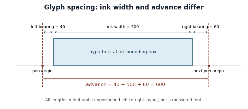
The right side bearing measures the signed gap from the right edge of a glyph's ink bounding box to the point specified by its default horizontal glyph advance. If the origin is $x=0$, the advance is $a$, and the ink edges are $x_L,x_R$, thenThus the advance splits into a left side bearing, an ink width and a right side bearing. OpenType uses this relation to derive the right side bearing from the horizontal metrics and outline bounds.^[ref]

For the hypothetical ink interval $40\le x\le 540$ and advance 600 font units, the right side bearing is 60 font units. If a different glyph extends to $x_R=650$ with the same advance 600, its right side bearing is $-50$ font units: ink crosses the next nominal origin. A negative bearing is therefore meaningful rather than an invalid width.

These are metrics of an individual default glyph. Kerning and other glyph positioning rules can change the actual gap between adjacent shapes, so the right side bearing alone does not determine the visual spacing of a whole run.

In a simple unpositioned horizontal layout, the left side bearing is the signed distance from a glyph's pen position to the left edge of its ink bounding box. Put the logical origin at $x=0$ and call the left ink edge $x_L$. Then $\mathrm{lsb}=x_L$. A positive value leaves space before the ink; a negative value means that the ink overhangs the origin.^[ref]

For example, a glyph whose ink occupies $40\le x\le 540$ and whose glyph advance is 600 font units has left side bearing 40, ink width 500 and right side bearing 60. These are default metrics; subsequent glyph positioning can change the rendered arrangement.

OpenType's horizontal-metrics table supplies the left side bearing and glyph advance. One must not assume that every outline's stored xMin is already the left side bearing: the outline's own coordinate origin and the metrics' logical origin need not coincide in every supported format.^[ref]

A syn glycosidic conformation is a base–sugar orientation in the syn region of the glycosidic torsion angle $\chi$. In the IUPAC-IUB convention the region is centered at $0^{\circ }$ and spans90degrees on either side. In a nonnegative360degree reporting interval, this region crosses the boundary: angles near both0 and360degrees belong to it.^[ref]

For an original example, $\chi =30^{\circ }$ and $\chi =330^{\circ }$ are both syn, because330degrees is equivalent to−30degrees. Their shortest angular separation is60degrees. Their ordinary arithmetic mean,180degrees, falls in the anti glycosidic conformation region and is therefore misleading as a mean orientation. Averaging their unit-circle vectors instead giveswhich points toward $\chi =0^{\circ }$.

The numerical convention is essential. Older choices using the base atom C8 for purines or C6 for pyrimidines can differ from the recommended glycosidic torsion angle by approximately180degrees. Comparing the same number under those two definitions could therefore appear to reverse a syn/anti assignment without any molecular motion.^[ref]

Syn is a local conformational descriptor. It is neither a statement that two bases are paired nor a label for the overall handedness of a nucleic-acid helix. Structural comparisons should retain the defining atoms and angle convention alongside the syn/anti label.

An anti glycosidic conformation is a base–sugar orientation in the anti region of the glycosidic torsion angle $\chi$. Under the IUPAC-IUB atom convention, this region is centered at $180^{\circ }$ and extends90degrees on either side. Equivalently, for an angle reported in $[0^{\circ },360^{\circ })$, the broad anti region lies between90 and270degrees.^[ref]

For a purine nucleoside, $\chi$ uses O4′–C1′–N9–C4; for a pyrimidine, it uses O4′–C1′–N1–C2. The ordered atoms specify the dihedral angle. An angle reported using different outer atoms cannot be assigned to this region by its numerical value alone.^[ref]

For an original example, $\chi =-160^{\circ }$ and $\chi =200^{\circ }$ describe the same orientation modulo one full turn, and both are anti. Moving to $\chi =60^{\circ }$ changes the orientation into the syn glycosidic conformation region while retaining the base–sugar bond connectivity. Conformational change and a change in covalent constitution are different descriptions.

The word anti here does not describe how two bases pair with one another. RNA base-pair geometry can separately classify the relative orientations of two glycosidic bonds. Nor does a single anti torsion determine the entire nucleotide or RNA structure: sugar geometry and the other backbone angles remain to be specified.