For the integer powers $p=2,3,4$, the Generalized Korteweg–De Vries equation is mass-subcritical. Its Gagliardo-Nirenberg interpolation inequality isThe exponent $\alpha =(p-1)/2$ is strictly below two. Since KdV mass and energy conservation fixes $\Vert u{\Vert }_2$ and $E(u)$, the gradient size $X=\Vert u_x{\Vert }_2$ obeys $X^2/2\le |E(u_0)|+C_{M(u_0)}{X}^{\alpha }$. Young's inequality for products absorbs the lower power into $X^2/4$ and leaves a uniform bound for $X$.

Under the standard local $H^1(\mathbb{R})$ solution theory with a continuation time controlled by the H1 norm, this bound extends the solution globally. At $p=5$, the nonlinear estimate has gradient exponent two, so this absorption argument requires additional information such as a small-mass threshold. The scaling identifies this as an L2 norm threshold.

The generalized tangent bundle of a smooth manifold $M$ is the direct sum of vector bundles $\mathbb{T}M=TM\oplus T^{\ast }M$. A fibre contains a tangent vector and a covector together. In real dimension $n$, it has rank $2n$ and a canonical symmetric bilinear formof signature $(n,n)$. No Riemannian metric is needed.^[ref]

Both $TM$ and $T^{\ast }M$ are isotropic: the pairing of any two elements of either summand is zero. A two-form $B$ gives the transformation $X+\xi \mapsto X+\xi +{\iota }_{X}B$. The new pairing terms sum to $B(X,Y)+B(Y,X)=0$, so the transformation preserves the pairing. These extra symmetries explain the utility of the bundle in generalized geometry, where complex structures and symplectic forms can be treated in one framework.

The untwisted skew-symmetric Courant bracket on sections of the generalized tangent bundle $TM\oplus T^{\ast }M$ isHere $[X,Y]$ is the Lie bracket of vector fields, $\mathcal{L}$ is the Lie derivative, and $d$ is the exterior derivative. It extends the Lie bracket of vector fields, but its Jacobi identity has an exact-form defect; it is not simply another Lie algebra bracket.^[ref]

For pure vector fields, $[X,Y{]}_C=[X,Y]$, and two pure one-forms have zero bracket. On the real line, $[{\partial }_x,f(x)dx{]}_C=\frac{1}{2}{f}^{\prime }(x)dx$. This mixed example shows how the bracket couples tangent and cotangent information through differentiation. Omitting the final exact term gives the nonskew Dorfman operation, a related convention with different identities.

Gear vibration order expresses the frequency of a measured vibration component relative to a specified shaft's rotation rate:Here $f$ is frequency in hertz and $n$ is shaft speed in revolutions per minute. The dimensionless order is cycles per shaft revolution. It must name the reference shaft: the same gear mesh frequency has different orders relative to the two gears in one mesh. Order tracking follows such rotation-related components as speed changes.^[ref]

For a24-tooth input at1500 revolutions per minute, $f_r=25\mathrm{Hz}$ and mesh frequency is600Hz, so mesh order is24. Its60-tooth mate turns at10Hz, giving mesh order60 relative to that shaft. If the input rises to1800 revolutions per minute, mesh frequency becomes720Hz but input-relative mesh order remains24. An unrelated structural natural frequency at600Hz would instead move from order24 to order20 as reference speed increases.

Angular resampling makes the distinction explicit. Let $\theta (t)=2\pi {\int }_0^t{f}_r(u)du$ be shaft angle. A tooth-periodic illustrative signal $a(t)=A\cos [N\theta (t)]$ can spread across many fixed-frequency bins during acceleration, while as a function of angle it remains $a(\theta )=A\cos (N\theta )$, with order $N$. Enough angle samples are needed to resolve the desired tooth-related oscillations. This derivation describes the resampling approach; not every order tracking algorithm uses that implementation.

Rotation-synchronous amplitude modulation can produce neighboring modulation sidebands: a24th-order component modulated once per input revolution has orders23 and25. Modulation associated with another shaft need not give integer spacing in the chosen reference. Orders identify kinematic relationships, while amplitudes still depend on loads, mounting and frequency response. A high mesh order or a sideband is therefore not itself a diagnosis of damaged teeth.^[ref]

A gear base circle is the fixed circle from which an involute tooth flank is generated. Imagining a taut string unwinding from that circle, the free end traces the involute. It is a geometric construction for the tooth shape, distinct from the gear reference circle used for sizing and the operating pitch circle describing a particular meshing pair.^[ref]

For base radius $r_b$ and unwinding parameter $u\ge 0$, one orientation of the involute isSquaring and adding gives $r=\sqrt{x^2+y^2}=r_b\sqrt{1+u^2}$. The local pressure-angle relation $\tan \alpha =u$ therefore gives $r_b=r\cos \alpha$. At the gear reference circle, this becomesFor reference diameter $d=60\mathrm{mm}$ and reference gear pressure angle $20{}^{\circ }$, the base diameter is $56.382\mathrm{mm}$, approximately. A change in mounting separation does not change this base diameter or the cut tooth profile; it changes which operating geometry describes the mesh.

In a compatible external pair, a common tangent to the two gear base circles is the gear line of action. Their fixed geometry gives $r_{b1}+r_{b2}=a\cos {\alpha }_w$, explaining why the operating pressure angle changes when $a$ changes. Repeating a tooth profile every $2\pi /N$ also gives gear base pitch $p_b=\pi d_b/N$ along the base circumference. Finally, an ideal involute generated this way lies on or outside its gear base circle; a real tooth's lower connecting portion can have a different shape. The gear base circle is not a physical boundary of the gear material.

A gear pitting inspection mask specifies the tooth-flank region over which damage is counted. It separates eligibility for inspection from the classification of an eligible location as pitted. The denominator of a gear pitting area fraction depends on this mask, so a change in coverage can change the reported fraction even when the surface has not changed.

For a digital image, let $m_i\in \{0,1\}$ indicate inclusion of pixel $i$ and let $p_i\in \{0,1\}$ indicate its classification as pitted. With represented surface area $a_i$ per pixel,The arrays $m_i$ and $p_i$ are different indicator functions. Uniform pixel areas cancel, but an oblique view or a curved-surface map can require nonuniform $a_i$. A shadow, occlusion or unrecorded region should not automatically count as intact material.

An original example begins with 200 pitted pixels among 10000 eligible equal-area pixels, giving $2\%$. Cropping to a 5000-pixel region that retains 150 pitted pixels gives $3\%$. The counted damaged area fell while the fraction rose; this comparison alone cannot establish damage growth.

A gear inspection common-region comparison first uses image registration to put inspections into corresponding surface coordinates. On a common grid, the intersection mask is $m_i^{\mathrm{common}}=m_i^{(0)}{m}_i^{(1)}$. Comparing the two pitting classifications within that same region holds the denominator convention fixed. Coverage outside the intersection should still be reported: excluding a newly obscured damaged edge can hide relevant change.

Useful inspection records retain the raw image, mask, geometric mapping, image thresholding or other image segmentation rule, and the reason for excluded regions. A primary NASA gear-endurance study combined inspection history with vibration and oil-debris observations, illustrating why damage labels must remain connected to actual inspected surfaces.^[ref] The mask formalism above is an explicit measurement convention, not a claim that every historical inspection used this pixel algorithm.

Gear normal pitch $p_n$ is the repeat spacing of corresponding helical gear tooth flanks normal to their tooth direction on the developed reference cylinder. It equals $\pi$ times gear normal module $m_n$. It is a different geometric spacing from gear transverse pitch $p_t$, measured circumferentially, and from gear axial pitch $p_x$, measured parallel to the rotation axis.^[ref]

Unwrap the reference cylinder into a plane. The equally spaced tooth traces become parallel straight lines making gear helix angle $\beta$ with the axis. Projecting the transverse spacing onto the normal to those traces givesFor reference diameter $d=60\mathrm{mm}$, $N=30$ teeth and $\beta =30{}^{\circ }$, $p_t=\pi d/N=2\pi \mathrm{mm}$, whereas $p_n=\sqrt{3}\pi \mathrm{mm}\approx 5.4414\mathrm{mm}$. Multiplying $p_n$ by $N$ gives about $163.24\mathrm{mm}$, not the $188.50\mathrm{mm}$ circumference: normal pitch is not the circumferential step.

At $\beta =0$, normal and transverse pitches agree, as expected for a spur gear. For nonzero gear helix angle, using one in place of the other introduces a factor $\cos \beta$. Normal pitch is also distinct from gear base pitch, which refers to the base-circle geometry of an involute. Matching a pitch value without its measurement convention, pressure angle and tooth geometry is insufficient to establish a compatible mesh.

The gear path of contact is the locus of actual tooth-contact points during an engagement. For a conventional external involute pair, its active part is a finite straight segment of the gear line of action. Its endpoints are set by the usable tooth flanks, rather than by the infinite geometric line alone. The part before the gear pitch point is the gear path of approach; the part after it is the gear path of recess in the stated direction of transmission.^[ref]

For a standard noninterfering external pair driven by gear1, let $r_{ai}$ be tip radii, $r_{bi}$ base radii, $r_{wi}$ operating radii and ${\alpha }_w$ the operating pressure angle. When tip circles bound the full usable contact,Adding gives $L=L_{\mathrm{app}}+L_{\mathrm{rec}}$. The two lengths need not be equal even when the gears use the same module and reference angle.

For the original module2,20/40-tooth example at20degree reference angle and60mm standard separation, tip radii22 and42mm give $L_{\mathrm{app}}\approx 5.0586\mathrm{mm}$ and $L_{\mathrm{rec}}\approx 4.5960\mathrm{mm}$. Their sum is $9.6546\mathrm{mm}$; dividing by gear base pitch $5.9043\mathrm{mm}$ gives transverse gear contact ratio about1.6352.

These are distances along the line of contact, not arc lengths traveled around a pitch circle. A shortened or altered flank can reduce the active interval, and interference can invalidate the full tip-limited construction. The labels approach and recess also depend on which direction is being followed. A practical contact inspection therefore needs the profile geometry and transmission direction, not just a sketch of two nominal pitch circles.

The gear pitch point is where the gear line of action meets the line joining the gear centers. For a fixed-axis external involute pair, it is the tangency point of the operating pitch circles. The point is a geometric location in the mesh, rather than a material mark permanently attached to one tooth.^[ref]

Let the gear centers be separated by $a$, with tooth counts $N_1,N_2$. Their operating radii locate the pitch point atFor external signed angular velocities, $r_{w1}{\omega }_1+r_{w2}{\omega }_2=0$. The two hypothetical material points occupying the pitch point therefore have the same instantaneous velocity. This is the local rolling without slipping property used to construct the operating pitch circles.

For an original example, use20 and40 teeth separated by $60\mathrm{mm}$. The pitch point is20mm from the first center and40mm from the second. With ${\omega }_1=50rad/s$ and ${\omega }_2=-25rad/s$, both surface velocities at that location have magnitude $1m/s$ and the same direction. Ideal relative gear sliding velocity is zero there.

Elsewhere on the gear path of contact, the two tooth surfaces can slide even while maintaining the required normal contact condition. The pitch point remains fixed in this fixed-axis geometry, while successive tooth-contact points advance through the mesh. Whether the pitch point itself belongs to a particular usable contact interval depends on the available flanks; the geometric definition does not assert that every modified tooth profile physically contacts at that point.

Gear tooth sliding is relative tangential motion of mating tooth surfaces at their contact point. Ideal contact prevents relative normal penetration but does not generally require the tangential surface velocities to agree. For a fixed-axis external involute pair, tangential slip vanishes at the gear pitch point and changes as the contact moves along the gear path of contact.^[ref]

Let $P$ be the pitch point, let $\mathbf{n}$ be a unit vector along the gear line of action, and write a contact location as $Q=P+s\mathbf{n}$. With a common positive axis $\hat{\mathbf{z}}$ and signed angular velocities ${\omega }_1,{\omega }_2$, rigid-body velocity differences giveThe velocities at $P$ cancel, leaving this term proportional to distance along the contact line. Since ${\omega }_2$ has opposite sign in an external pair, the sliding-speed magnitude is $(|{\omega }_1|+|{\omega }_2|)|s|$.

For an original example, use ${\omega }_1=50rad/s$ and ${\omega }_2=-25rad/s$. At $s=4\mathrm{mm}$, gear sliding velocity along the common tooth tangent is $0.30m/s$; at $s=-4\mathrm{mm}$ it has the opposite sign. At $s=0$ it is zero. Equality of operating pitch-circle speeds must therefore not be used to conclude that the tooth flanks roll without slipping throughout engagement.

In a simplified Coulomb friction model with coefficient of friction $\mu$ and normal load $F_n$, the dissipated gear sliding-friction loss is $P_f=\mu F_n|v_s|$. Hypothetical values $\mu =0.05$, $F_n=100\mathrm{N}$ and $|v_s|=0.30m/s$ give $1.5\mathrm{W}$. This is a local illustrative loss model, not a lubricant specification. Zero ideal sliding at the pitch point also does not eliminate every source of gearbox loss, such as support friction or deformation-related dissipation. Real load and friction can vary through the engagement, so total loss requires integrating the applicable contact model.

Gear lead $L$ is the axial advance of one tooth helix over a complete turn around a cylindrical helical gear. It differs from gear axial pitch $p_x$, which steps between successive teeth at one circumferential position. With $N$ equally spaced tooth helices, $L=N{p}_x$. The lead magnitude does not specify whether the helix is right-handed or left-handed.^[ref]

Unwrapping a reference cylinder of diameter $d$ gives a right triangle with axial side $L$ and circumferential side $\pi d$. Since gear helix angle $\beta$ is measured from the axis,For $d=60\mathrm{mm}$ and $|\beta |=30{}^{\circ }$, $L=60\pi \sqrt{3}\mathrm{mm}\approx 326.484\mathrm{mm}$. If $N=30$, then gear axial pitch is $10.8828\mathrm{mm}$; confusing the two distances would introduce a factor30.

A useful geometric check keeps the lead fixed while changing the chosen concentric cylinder. The helix's axial advance per revolution remains $L$, but its angle satisfies $\tan |\beta (r)|=2\pi r/L$. For the same lead on diameter $40\mathrm{mm}$, the angle is approximately $21.052{}^{\circ }$, rather than $30{}^{\circ }$. Thus a helix-angle specification needs its cylinder, normally the reference cylinder. Lead can remain finite when the physical tooth is much shorter than one complete turn: it describes the continued helix, not a requirement that the manufactured tooth cover a full revolution.

Gear axial pitch $p_x$ is the axial repeat distance between corresponding flanks of successive teeth of a cylindrical helical gear. The measurement follows a line parallel to the rotation axis on a concentric cylinder. It is not the axial advance of one tooth helix through an entire revolution; that larger distance is gear lead $L$. For $N$ equally spaced teeth, $L=N{p}_x$.^[ref]

On the developed cylinder, neighboring tooth traces separated transversely by gear transverse pitch $p_t$ intersect a fixed circumferential coordinate at axial positions separated by $p_x$. Their slope givesFor $d=60\mathrm{mm}$, $N=30$ and gear helix angle $|\beta |=30{}^{\circ }$, $p_t=2\pi \mathrm{mm}$ and $p_x=2\pi \sqrt{3}\mathrm{mm}\approx 10.8828\mathrm{mm}$. The corresponding gear normal pitch is only $5.4414\mathrm{mm}$. These two distances differ by a factor of two in this example because $\sin 30{}^{\circ }=1/2$.

For an engaged gear face width $b=20\mathrm{mm}$, the ideal gear overlap ratio is $b/p_x\approx 1.8378$: successive tooth-contact traces span about1.84 axial pitches across the face. Holding $p_t$ fixed while letting $\beta$ tend to zero makes $p_x$ diverge. Straight spur gear tooth traces do not cross an axial generator successively, so a finite axial-pitch interpretation does not survive that limit. Helix hand determines orientation; the positive pitch magnitude alone does not specify hand.

A gear face load factor quantifies the effect of nonuniform load across the engaged gear face width. For the contact-load convention in ISO 6336-1:2006, $K_{H\beta }$ compares maximum line-load intensity with the mean intensity over the stated width:Here $F_m$ is the total load represented by that distribution and $b$ is its evaluation width. A uniform distribution gives1; an edge-concentrated distribution gives a larger value. The numerator and denominator must refer to the same load convention and operating condition.^[ref]

For an original illustrative distribution over $b=20\mathrm{mm}$,total load is1000N, mean line load is50N/mm and maximum line load is80N/mm. Thus $K_{H\beta }=1.6$. A uniform distribution with the same width and total load gives1. The gear contact pattern can cover the whole width in both cases.

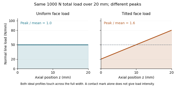
For ideal elastic line contact at fixed geometry and material, Hertzian contact pressure scales with the square root of line load. The corresponding gear contact-stress load factor is therefore $\sqrt{1.6}\approx 1.265$ in this simplified comparison. Multiplying the contact pressure itself by1.6 would confuse a load-intensity ratio with a stress ratio. This scaling does not replace a complete gear-rating calculation.

The manufacturer's treatment connects face-load assessment to shaft-support placement, shaft stiffness and loaded contact quality.^[ref] A value inferred from a toy line-load profile is consequently useful for understanding the factor, while a real design must obtain the relevant distribution or factor from a method appropriate to its geometry and load state.

A gear contact pattern is the observed region of tooth-flank contact during a stated mesh test. Its position and extent reveal how the installed tooth surfaces meet. A gear contact marking test uses a thin marking layer and controlled rotation to make that region visible; the mounting position, transmission direction and applied torque belong in the test description. Manufacturer guidance treats surface-contact checks as evidence about the assembled mesh, including shaft alignment.^[ref]

A useful bench comparison holds the gear pair and test conditions fixed, records the initial mark, then changes one alignment setting and repeats the test. A mark moving toward one face edge indicates a change in where the flanks meet. This is an observation of contact location, rather than an automatic measurement of operating pressure or a universal diagnosis of the alignment error.

For example, a mark occupying the full20mm gear effective face width is compatible with a hypothetical uniform line load $w=50N/mm$, but also with the tilted positive distributionBoth integrate to1000N, yet their peak line loads are50 and80N/mm. Merely observing full-width contact cannot choose between those gear face load distributions. The gear face load factor or local stress needs additional load/deformation information.

Loaded and lightly loaded patterns can also differ because shaft, housing and tooth deformation change the gap. A quantitative loaded assessment may use strain measurements or a validated contact model alongside the pattern; the2006 gear-rating standard explicitly distinguishes comprehensive load assessment from the limited information in a bearing pattern.^[ref]

Gear base pitch is the spacing of successive involute tooth profiles referred to the gear base circle. For base diameter $d_b$, tooth count $N$, gear module $m$ and reference gear pressure angle $\alpha$,It also gives the spacing between successive corresponding tooth contacts measured along the gear line of action. The gear circular pitch uses the reference circle instead, giving $p=\pi m$ and $p_b=p\cos \alpha$.^[ref]

For $m=2\mathrm{mm}$ and $\alpha =20{}^{\circ }$, $p=6.2832\mathrm{mm}$ but $p_b\approx 5.9043\mathrm{mm}$. A second gear with the same module but $25{}^{\circ }$ reference angle has $p_b\approx 5.6945\mathrm{mm}$. Matching reference tooth spacing alone therefore does not make these the same specified mating geometry.

Changing the mounting separation of a compatible involute pair does not change its cut profiles, base circles or gear base pitch. In operating-circle notation, $p_w=2\pi r_w/N$ changes with mounted radius, whilestays fixed. This links the mounted operating pressure angle to an invariant tooth-profile spacing.

For a tooth rotating at angular speed $\omega$, base-circle tangential speed is $r_b|\omega |$. Dividing by gear base pitch gives the gear mesh frequency,A 30-tooth gear at $600$ revolutions per minute gives $f_m=300\mathrm{Hz}$. Finally, the gear contact ratio divides usable gear path of contact length by this base pitch, so profile spacing and available contact length jointly determine overlap between successive tooth engagements.

The Gouy phase describes the additional axial phase associated with a focused wave relative to a plane wave. For a fundamental circular Gaussian beam with beam waist at $z=0$ and Rayleigh range $z_R>0$, defineWith the carrier convention $e^{i(kz-\omega t)}$, the on-axis field phase is $kz-\omega t-\psi (z)$ up to a constant. Thus the signed additional phase is $-\psi$ in this convention; defining the positive function $\psi$ does not reverse the physical prediction.^[ref]

The complex field prefactor gives a short derivation. The normalized Gaussian propagation factor isIts modulus describes the on-axis amplitude reduction; its argument is the additional phase. An intensity measurement alone loses this argument, so measuring the beam's width and brightness does not directly measure the Gouy phase.

As $z$ runs from far before to far after the waist, $\psi$ runs continuously from $-\pi /2$ to $+\pi /2$. The total additional phase change has magnitude $\pi$, but is not a discontinuous jump at the waist. For stipulated $w_0=100\mu \mathrm{m}$ and $\lambda =633\mathrm{nm}$, $z_R\approx 49.6\mathrm{mm}$. Between $z=-z_R$ and $z=+z_R$, the additional phase changes by $-\pi /2$; the far-field-to-far-field limit gives $-\pi$.

The number of confined transverse directions matters. A Gaussian beam with one transverse coordinate has prefactor $(1+iz/z_R{)}^{-1/2}$ and half this phase contribution. Simin Feng and Herbert G. Winful's primary analysis relates the effect to transverse confinement and the angular spectrum representation: a localized beam includes transverse wave-vector components, affecting axial propagation.^[ref]

An illustrative Gouy phase interferometry experiment overlaps the focused beam with a coherent reference beam and records the interference phase at different axial planes. Removing the ordinary optical-path contribution and accounting for wavefront curvature isolates the axial phase change. This is a proposed measurement outline, not an experimental result reported by the cited theoretical paper. In an optical cavity, related phase contributions help determine the resonance condition and distinguish transverse modes.

Fourier localization of a Gaussian beam expresses the tradeoff between a narrow transverse field and a broad distribution of transverse spatial frequencies. At a waist, takeTwo Gaussian integrals giveReducing $w_0$ therefore broadens the angular spectrum method representation rather than merely shrinking a picture in the same set of propagation directions.^[ref]

Widths must state their weighting. Normalize $|U{|}^2$ and $|\tilde{U}{|}^2$ to define transverse position and transverse-wavenumber distributions. Their one-coordinate standard deviations areThese are optical field-width statements under the stated Fourier convention, not an inference that each ray has simultaneously measured position and angle. Using amplitude widths instead would give different numerical factors.

For a strongly paraxial spectrum, ${\theta }_x\simeq k_x/k$ and ${\sigma }_{{\theta }_x}=1/(k{w}_0)$. The usual far-field Gaussian $1/e^2$ light intensity half-angle is $2{\sigma }_{{\theta }_x}=\lambda /(\pi w_0)$. For original $\lambda =632.8$ nm and $w_0=0.50$ mm, ${\sigma }_x=0.25$ mm and ${\sigma }_{{\theta }_x}\simeq 0.2014$ mrad; the conventional divergence half-angle is about 0.4029 mrad. Halving the waist doubles both angular measures.

An illustrative apparatus places a camera in a plane conjugate to the waist and another measurement at a lens's back focal plane, where transverse spatial frequency maps to position in the paraxial model. Comparing widths tests localization and angular spread, provided magnification, focal length and detector response are accounted for. Finite aperture clipping changes the field and produces extra spectral structure, so the exact Gaussian width product cannot simply be assigned to every clipped beam.

The same spectrum also bounds the paraxial approximation: $k{w}_0\gg 1$ keeps most amplitude at transverse wavenumbers much smaller than $k$. Strong focusing can require vector polarization constraints and a nonparaxial propagation model.

Wringing-film uncertainty is the uncertainty contributed by differences or changes in the effective contact layers formed during gauge block wringing. Because the defined length of a gauge block includes a wringing-layer convention, the issue is the difference between calibration and use, not automatically an extra layer correction added to every certificate value.

For a stack of $n$ blocks wrung to an auxiliary plane, let $w_i$ denote each calibrated effective layer contribution and $w_j^{\prime }$ the contributions from the $n-1$ internal contacts plus the base contact in use. The residual contact correction isIts standard uncertainty requires a model for these differences. NIST's handbook describes dependence on surface condition, fluid and elapsed time, and notes residual uncertainty when an unknown block's layer is transferred through comparison with a master.^[ref]

An original model for $n$ effective contact differences writes ${\delta }_j=b+{ϵ}_j$, with one shared zero-mean contribution $b$ of variance $u_b^2$ and independent contact contributions ${ϵ}_j$ of variance $u_{ϵ}^2$. ThenThe common term grows quadratically in variance because every contact contains the same contribution. Treating all contacts as independent would omit their covariance.

For three contacts with stipulated $u_b=3\mathrm{nm}$ and $u_{ϵ}=2\mathrm{nm}$, the combined standard uncertainty is $\sqrt{9\cdot 9+3\cdot 4}=\sqrt{93}\approx 9.64\mathrm{nm}$. Assuming independence for three marginal uncertainties $\sqrt{13}\mathrm{nm}$ instead gives $\sqrt{39}\approx 6.24\mathrm{nm}$. The numerical difference comes entirely from the assumed shared effect; these values are illustrative, not a general wringing specification.

Repeatedly separating, preparing and rewringing contacts can characterize a repeatability contribution. Repeated detector readings of an unchanged stack do not sample new wrings. Averaging independent rewrings may reduce a random contact term while leaving a shared calibration or preparation contribution. Film evolution and thermal expansion during handling must also be distinguished from readout noise.

Report surface preparation, reference geometry, elapsed time and the treatment of shared effects. A stack that adheres firmly can still have a length contribution relevant to a small uncertainty target. Wringing-film covariance model assumptions therefore belong with the result, rather than being hidden inside an unspecified repeatability number.

Differential thermal-expansion uncertainty is the uncertainty in the unequal thermal length changes of two compared objects. In a gauge-block thermal mismatch correction, shared temperature and coefficient information determine which contributions cancel and which remain.

For approximately equal known nominal length $L$, coefficient difference $a={\alpha }_X-{\alpha }_R$ and common temperature offset $\theta =T-T_0$, the differential correction is $d=La\theta$. Its first-order sensitivity coefficients are $\partial d/\partial a=L\theta$ and $\partial d/\partial \theta =La$. HenceLength uncertainty and other inputs require further terms when they are material to the result. General propagation must retain input covariance.^[ref]

The coefficient difference itself hasAssuming two coefficient estimates independent merely because two blocks are present can therefore misstate the uncertainty. Similarly, a common thermometer contribution is not two unrelated temperature errors. NIST's handbook explicitly treats differences in block temperatures and expansion coefficients in comparisons.^[ref]

An original example takes $L=100\mathrm{mm}$, $a=6.5\times 10^{-6}{\mathrm{K}}^{-1}$, $\theta =2\mathrm{K}$, independent $u(a)=0.5\times 10^{-6}{\mathrm{K}}^{-1}$ and $u(\theta )=0.1\mathrm{K}$. The correction is $1.3\mu \mathrm{m}$. The two first-order standard-uncertainty contributions are 0.10 and $0.065\mu \mathrm{m}$, giving combined $u(d)\approx 0.119\mu \mathrm{m}$. These are stipulated inputs, not a certificate.

A useful boundary case exposes second-order thermal mismatch uncertainty. If both central values $a$ and $\theta$ are zero, the linear sensitivities vanish even though both inputs remain uncertain. For independent inputs with those means, their product has exact variance $L^2{u}^2(a)u^2(\theta )$. With $L=100\mathrm{mm}$, $u(a)=10^{-6}{\mathrm{K}}^{-1}$ and $u(\theta )=0.1\mathrm{K}$, this gives 10 nm standard uncertainty, while first-order propagation gives zero. The GUM explicitly requires attention to higher-order terms when nonlinearity matters.^[ref]

Specify the thermal model, shared inputs and approximation used. A small nominal correction is not automatically evidence that its uncertainty is negligible.

Shared gauge-block reference covariance is the dependence between calibrated length estimates caused by using the same uncertain reference. It explains how a gauge-block reference uncertainty floor can remain in individual absolute lengths while canceling from their difference.

Let corrected estimates be $X=R+d_X$ and $Y=R+d_Y$. Suppose the shared reference error has variance $u_R^2$, the comparison errors have variances $u_X^2,u_Y^2$, and these three contributions are independent. The covariance matrix isIn particular, $\mathrm{cov}(X,Y)=u_R^2$. The covariance follows from the shared input, rather than from whether the two comparison readings happened at the same instant.

For the contrast $D=X-Y$,Both reference sensitivities are exactly one in this additive measurement model, so their contributions cancel. General uncertainty propagation includes precisely this covariance term.^[ref]

An original example uses $u_R=20\mathrm{nm}$, $u_X=10\mathrm{nm}$ and $u_Y=15\mathrm{nm}$. The individual standard uncertainties are about 22.36 and 25 nm, while the difference has standard uncertainty $\sqrt{100+225}\approx 18.03\mathrm{nm}$. Incorrectly treating the absolute length estimates as independent would give $\sqrt{500+625}\approx 33.54\mathrm{nm}$ for the same difference.

For any linear combination $Z=c_{X}X+c_{Y}Y$, the reference contribution is $u_R^2(c_X+c_Y{)}^2$. It vanishes for a difference but remains $u_R^2$ in an equal-weight average, where $c_X=c_Y=1/2$. Repeatedly averaging values carrying the same reference error does not produce independent reference information.

Unequal gauge-block reference sensitivities change the cancellation. If the reference enters as $a_{X}R$ and $a_{Y}R$, a difference retains reference variance $(a_X-a_Y{)}^2{u}_R^2$. Shared temperature, comparator or wringing contributions also need their own coefficients and dependence assumptions. NIST's uncertainty procedure separates the master history from comparison-process variability.^[ref]

Retain the calibration lineage and input relationships with the estimates. A pair of certificate uncertainty numbers alone does not establish their covariance or justify setting it to zero.