Topics (384k) Articles (398k) Users (410) Discussions (242) Comments (383) Files (13k) New article

For a cost-minimization game, the price of anarchy is the ratio of the worst equilibrium social cost to the best feasible social cost:Here is the specified equilibrium set, the feasible profiles, and the chosen nonnegative social cost. The ratio requires a positive denominator; zero optimum costs and empty equilibrium sets need separate conventions. A payoff-maximization formulation uses the reciprocal orientation to keep a larger number meaning worse efficiency.
In the two-edge routing game with one unit of flow and latencies and one, the equilibrium costs one while the optimum costs , so the price of anarchy is . The best equilibrium instead defines the price of stability. Bounds depend on the equilibrium notion and the allowed game class; one example does not establish a universal bound for all games.
For a cost-minimization game with positive social optimum and a nonempty set of the specified Nash equilibria, the price of stability isIt measures the cost of requiring stability even when the best equilibrium can be selected. The equilibrium class, such as pure or mixed, and social-cost convention must be stated.
In a symmetric two-player game with actions , let each player's cost be one at , two at and three when the actions differ. Both coordinated choices are Nash equilibria; the best equilibrium has total cost two, matching the optimum, so the price of stability is one. The worst equilibrium instead costs four, giving price of anarchy two. The distinction matters when a designer can recommend an outcome but cannot force anyone to remain at an unstable one.[ref]
The Price of Stability for Network Design with Fair Cost Allocation by Elliot Anshelevich and others. Introduction, best equilibrium and stability interpretation
A complex algebraic variety is an algebraic variety over the complex numbers. In the scheme convention used here, it is a reduced separated scheme of finite type over ; irreducibility is an additional condition when needed. Affine examples are zero sets of complex polynomials equipped with their regular functions.
For example, is the union of two complex coordinate lines, while is an irreducible singular curve. The smooth locus of a complex variety has the structure of a complex manifold, but a singular point need not be smooth as a complex analytic space.
One must also distinguish topologies. The complex affine line is as a point set; its proper Zariski-closed subsets are finite, whereas its usual analytic topology has many more closed and open subsets. Passing from an algebraic variety to its analytic space retains geometric information while changing which local functions and open sets are allowed.
For a projective variety , its secant variety is the Zariski closure of the union of projective lines joining distinct points of . More generally is the closure of the spans of points. Taking the closure includes limiting configurations; it is essential to the definition.[ref]
For a nonsingular conic in the Complex projective plane, secants fill a dense subset of the plane and their closure is the entire plane. As the two points merge, a secant line tends to a tangent line. For tensor rank problems, sums of decomposable tensors give secant constructions; the closure also permits limits of such sums. This is why secant geometry naturally describes border rank, which can be smaller than actual tensor rank.
Over an algebraically closed field , a rational surface is an algebraic surface birational to the projective plane . Equivalently its function field is isomorphic to , a purely transcendental extension of degree two. The birational maps need only be inverse on dense open subsets.
The product is rational: it contains the affine plane as the product of two affine charts, and also contains the affine plane. Blowing up a point on a smooth rational surface preserves its function field, hence its rationality, while changing its curves and intersection geometry.
Rationality is consequently weaker than being isomorphic to . It is also a geometric condition on the whole surface, rather than an assertion that every point has rational-number coordinates. Over a non-algebraically-closed field, the field over which the birational map is defined must be specified.
An airfoil thickness convention specifies which two surface points are paired, the direction used to measure their separation and how the result is normalized. An airfoil thickness-to-chord ratio is reproducible only after these choices are fixed. A vertical gap at common chordwise coordinate is not generally the same quantity as thickness constructed normal to a sloping airfoil mean camber line.
For the NACA four-digit airfoil construction, let a mean-line station be , its tangent make angle with the airfoil chord, and the prescribed half-thickness be . The paired upper and lower points satisfyTheir separation vector is , with Euclidean norm . Their chordwise coordinates differ when the mean line slopes. These normal offsets are the construction specified in the originating aerodynamic geometry notes.[ref]
Two different vertical measurements must also be distinguished. The vertical component of that paired separation is . A vertical line cutting two locally parallel straight surfaces instead spans . For an original local model with true normal thickness 10 mm and , these values are 8.660 mm and 11.547 mm, respectively. The first projects a selected segment; the second intersects surfaces at a common horizontal coordinate. For curved surfaces, the actual intersection must be calculated rather than assuming the local straight-line approximation is exact.
At a zero-slope station the three quantities coincide. This explains why a maximum-camber example can conceal a convention difference that becomes visible elsewhere. Taking the maximum over a profile also requires stating which thickness function is being maximized; a family designation is not a complete recipe for every possible projected maximum.
A coordinate-based geometry check should therefore retain the airfoil chord, mean-line rule, surface pairing and measurement direction. A photograph adds a further projection problem unless its viewing direction and scale are controlled. These are geometric qualifications; choosing a thickness convention does not by itself predict lift, drag or aerodynamic stall.
The mean aerodynamic chord is a reference length that weights each local airfoil chord by the area of its spanwise strip. For a symmetric aircraft wing with wingspan , local chord and wing area , its geometric definition isThe extra factor of distinguishes this from the mean geometric chord .[ref]
The weighting has a simple interpretation: a strip has area , so is an area-weighted mean. If a simplified section model has the same local pitching moment coefficient and dynamic pressure everywhere, its strip moment is . Integration then gives . This explains its use as a moment reference; an actual three-dimensional flow need not have a uniform section coefficient.
For the mean aerodynamic chord of a trapezoidal wing, take root chord , tip chord and a linear distribution . Integrating givesThe stipulated wing planform , , has , and . The wider strips receive more weight.
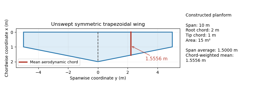
Trapezoidal wing planform with a mean aerodynamic chord of 1.5556 m, compared with the span-average chord of 1.5 m. Original geometry calculation.
Details. The Cauchy-Schwarz inequality gives a useful general check:Equality holds for a constant chord almost everywhere. A reported mean aerodynamic chord shorter than therefore contradicts this definition for the same span and area convention. Its length alone does not specify a location: the reference position of that chord and the aerodynamic center are additional geometric or aerodynamic data.
The mean geometric chord, also called the standard mean chord, is the span-average airfoil chord of an aircraft wing:where is the wing area and the wingspan. The area is the projected wing planform, not the sum of the upper and lower skin areas.[ref]
A useful exact identity explains its difference from the mean aerodynamic chord. Represent uniform spanwise averaging by a coordinate with a continuous uniform distribution on , and put . This is a mathematical averaging device, not a claim that the wing geometry is random. With ,Thus the relative excess is the squared coefficient of variation of the local chords. The mean aerodynamic chord can also be interpreted as the expected value under the corresponding size-biased distribution, since larger chords receive proportionally larger weights.
For the original linear taper from to , uniform spanwise sampling makes uniform on . Its expected value is and variance is . Hence , a relative excess of . A constant-chord wing has zero variance, so its two averages coincide.
Equal does not determine how local chord varies or where the wing lies relative to a reference axis. Those additional data enter wing sweep and the mean aerodynamic chord reference position.
A pneumotachograph measures and records gas volumetric flow rate from the pressure difference produced across a resistive flow head. In a mesh-type implementation, two pressure taps sample opposite sides of a fine screen, and tubing connects them to a differential pressure sensor. The flow head need not contain electronics; the pressure transducer and amplifier convert its response to a recorded signal. The manufacturer manual documents this arrangement and limits proportionality to an appropriate flow range.[ref]
Front-end Signal Conditioners Owner’s Guide. Chapter 10, printed p. 149, Using the Spirometer, Figure 10–6
For an original quasisteady linear model, let signed volume flow rate be , head hydraulic resistance for the specified gas and conditions, and pressure-drop convention for a fixed positive direction. ThenHere is the pressure-to-output gain and the zero-flow offset. Reversing flow reverses the modeled pressure difference. The pressure taps retain fixed labels when direction changes; renaming them upstream and downstream on each reversal would discard the sign.
A bundle of identical long circular capillaries gives an illustrative viscous model,under the assumptions of fully developed laminar flow, negligible compressibility and negligible entrance losses. This Poiseuille flow calculation explains one way to obtain an approximately linear pressure/flow relation. It is not an exact geometry model for every mesh head. Changes in gas viscosity, contamination, leakage or nonlinear inertial losses can change the calibration.
For a numerical signal-chain example, choose and . A flow of produces and an offset-corrected output of . If this flow lasts two seconds, the transported volume is . The head also adds a real pressure drop to the gas path; a sensitive measurement can therefore alter the system being measured.
Zero-offset drift of an integrated flow measurement follows directly from time integration. For inferred flow with constant offset ,An offset of accumulates of volume error in thirty seconds. Zeroing the no-flow signal addresses this additive contribution; it does not establish the flow scale. The manual treats zeroing and known-volume calibration separately.[ref]
Front-end Signal Conditioners Owner’s Guide. printed pp. 151–153, Calibrating the Flow Head and Reducing Drift
A proposed bench calibration connects a known-displacement piston or calibration syringe, records the output and verifies that its integral recovers the displaced gas volume under the stated conditions. Repeat several piston speeds and both directions. Agreement for one integral does not prove the instantaneous waveform is accurate: pressure-tap tubing, amplifier filters and sensor dynamics can distort fast changes while preserving an overall area approximately.
For a measured integral and known displaced volume , the linear conversion factor is , so . State the volume’s pressure and temperature conditions, and test the intended rate range before extending that factor. The manufacturer’s known-volume syringe procedure supplies this physical calibration principle.[ref]
Front-end Signal Conditioners Owner’s Guide. printed pp. 151–152, Injecting a known volume and integrating
Calibration establishes the response of the complete gas-flow measurement chain under its tested conditions. Pinned article: Introduction to the OurBigBook Project
Welcome to the OurBigBook Project! Our goal is to create the perfect publishing platform for STEM subjects, and get university-level students to write the best free STEM tutorials ever.
Everyone is welcome to create an account and play with the site: ourbigbook.com/go/register. We belive that students themselves can write amazing tutorials, but teachers are welcome too. You can write about anything you want, it doesn't have to be STEM or even educational. Silly test content is very welcome and you won't be penalized in any way. Just keep it legal!
Intro to OurBigBook
. Source. We have two killer features:
- topics: topics group articles by different users with the same title, e.g. here is the topic for the "Fundamental Theorem of Calculus" ourbigbook.com/go/topic/fundamental-theorem-of-calculusArticles of different users are sorted by upvote within each article page. This feature is a bit like:
- a Wikipedia where each user can have their own version of each article
- a Q&A website like Stack Overflow, where multiple people can give their views on a given topic, and the best ones are sorted by upvote. Except you don't need to wait for someone to ask first, and any topic goes, no matter how narrow or broad
This feature makes it possible for readers to find better explanations of any topic created by other writers. And it allows writers to create an explanation in a place that readers might actually find it.
Figure 1. Screenshot of the "Derivative" topic page. View it live at: ourbigbook.com/go/topic/derivativeVideo 2. OurBigBook Web topics demo. Source. - local editing: you can store all your personal knowledge base content locally in a plaintext markup format that can be edited locally and published either:This way you can be sure that even if OurBigBook.com were to go down one day (which we have no plans to do as it is quite cheap to host!), your content will still be perfectly readable as a static site.
- to OurBigBook.com to get awesome multi-user features like topics and likes
- as HTML files to a static website, which you can host yourself for free on many external providers like GitHub Pages, and remain in full control

Figure 2. You can publish local OurBigBook lightweight markup files to either OurBigBook.com or as a static website.
Figure 3. Visual Studio Code extension installation.
Figure 5. . You can also edit articles on the Web editor without installing anything locally. Video 3. Edit locally and publish demo. Source. This shows editing OurBigBook Markup and publishing it using the Visual Studio Code extension. 
- Infinitely deep tables of contents:



All our software is open source and hosted at: github.com/ourbigbook/ourbigbook
Further documentation can be found at: docs.ourbigbook.com
Feel free to reach our to us for any help or suggestions: docs.ourbigbook.com/#contact