The minimal polynomial $m_T$ is the unique monic polynomial of least degree with $m_T(T)=0$. Existence follows from a linear dependence among powers of $T$ in the finite-dimensional vector space $\mathrm{End}(V)$; polynomial division proves uniqueness and that it divides every annihilating polynomial. The characteristic polynomial is ${\chi }_T(t)=\det (tI-[T{]}_{\mathcal{B}})$, independent of basis because a change of basis conjugates the matrix.

WriteIn the cyclic basis, the companion matrix isFor $q(t)=t^n+a_{n-1}{t}^{n-1}+\cdots +a_0$, the displayed vector relation gives $q(T)v=0$. Polynomial evaluation commutes with $T$, so $q(T)T^{j}v=T^{j}q(T)v=0$ for every basis vector. Thus $q(T)=0$.

No nonzero polynomial of degree below $n$ can annihilate $T$, since applying it to the cyclic vector $v$ would contradict independence of $v,Tv,\dots ,T^{n-1}v$. Hence $m_T=q$. Finally, direct expansion of $\det (tI-C)$, or induction along the last column, gives ${\chi }_T(t)=t^n+a_{n-1}{t}^{n-1}+\cdots +a_0=q(t)$. ThereforeThe argument computes the determinant and annihilator directly and does not invoke the Cayley-Hamilton theorem.

The second equilibrium point equation gives $y=-(x+1)/2$. Substituting into the first gives $x+e^{(x-1)/2}=0$, so $x<0$. Put $x=-a$, with $a>0$. ThenThe function $h(a)=a{e}^{(a+1)/2}$ is strictly increasing on $a\ge 0$, since $h^{\prime }(a)=e^{(a+1)/2}(1+a/2)>0$. It starts at zero and tends to infinity, so it takes the value one exactly once. Moreover $h(1)=e>1$, so $0<a<1$. This proves uniqueness of the stated equilibrium point.

At that point $e^{x+y}=a$, and the Jacobian matrix isIts trace is $3+a$ and determinant $2+a$. The characteristic discriminant is $(3+a{)}^2-4(2+a)=(a+1{)}^2$, so its two eigenvalues areThey are distinct and positive, with eigenvectors $(1,-1)$ and $(a,1)$ respectively. Thus the linearized critical point is an unstable node. It is a hyperbolic equilibrium, so the original nonlinear equilibrium point is also locally repelling; this last observation is stronger than the requested linearized classification.

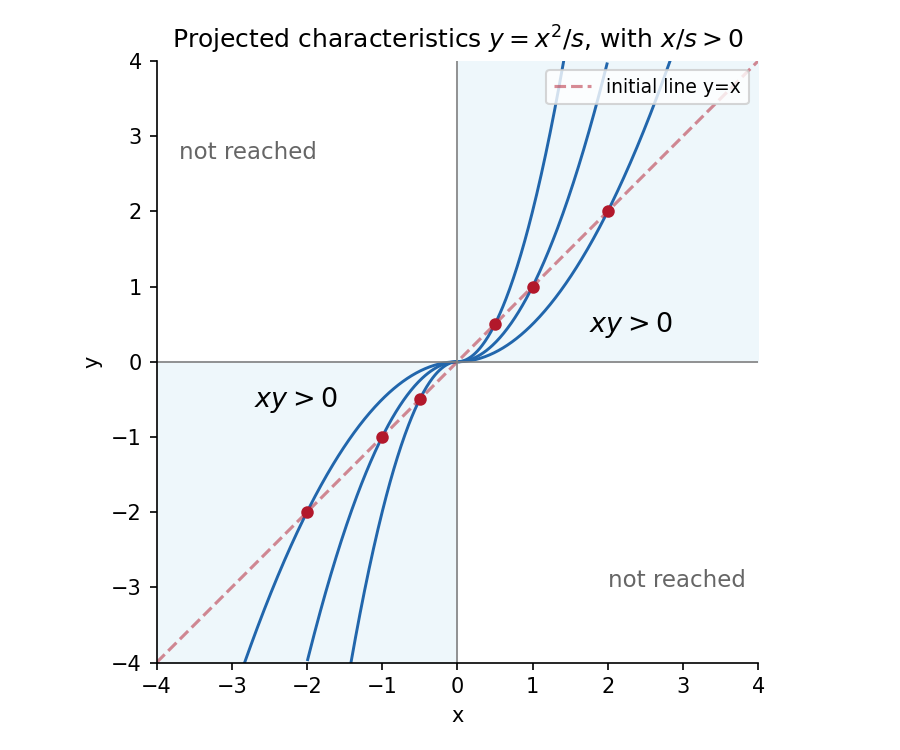
Choose characteristic parameter $t$ with initial value at $t=0$. The characteristic equations areThe first two integrate immediately; substitution into the third givesEliminating $t$ gives the projected parabolaThe sign restriction selects the half-parabola actually reached from the initial point.

The projection map $(s,t)\mapsto (s{e}^t,s{e}^{2t})$ has Jacobian determinant $s{e}^{3t}\ne 0$, so the initial curve is noncharacteristic for every allowed $s$. Its global inverse isdefined precisely when $x,y$ have the same nonzero sign. Every such point is reached by exactly one characteristic. Hence the region of unique determination from these initial data projects ontothe first and third quadrants. The axes are not reached for finite parameter from $s\ne 0$, and the other two quadrants have no method of characteristics issued from this initial curve.

As a direct check, substitution of the inverse parameters gives the solutionIt has $z(s,s)=s^2$, and differentiating gives $x{z}_x+2y{z}_y=xy$. This is quadrant uniqueness for unequal dilation characteristics.

For $y=\alpha x+\beta x^2$, the derivatives are $y^{\prime }=\alpha +2\beta x$ and $y^{\prime \prime }=2\beta$. Substituting gives $2\beta x^2-2x(\alpha +2\beta x)+2(\alpha x+\beta x^2)=0$. The independent solutions $x,x^2$ have Wronskian $x^2\ne 0$ on $[1,2]$, so they form a fundamental system of solutions.

Divide the inhomogeneous linear differential equation by $x^2$ and use variation of parameters. Choosing integrals from one gives the particular solutionThus $z=Ax+B{x}^2+z_p$. The first boundary condition gives $A=-B$. The integral endpoint terms cancel when differentiating $z_p$, so the second givesConsequentlyCollect the coefficient of $f(t)$ on either side of $t=x$. A suitable Green function isThe two pieces agree at $x=t$, $G(1,t)=0$, and $G_x(2,t)=0$ for $t<2$. For an interior source point its derivative jump isThus multiplication by the leading coefficient $t^2$ gives unit in a ring source strength. Away from $x=t$, both pieces solve the homogeneous linear differential equation. With continuous $f$, the integral representation has the required second derivative and solves the equation pointwise in $(1,2)$.

For uniqueness, the difference of two solutions is $Ax+B{x}^2$. Its boundary conditions give $A+B=0$ and $A+4B=0$, forcing $A=B=0$. Hence the solution is unique. This is the mixed Green function for an Euler operator with exponents one and two.

A function on the open set $D$ is holomorphic if at every $a\in D$ the complex limitexists. The limit is independent of the direction of approach.

A pole of order $n\ge 1$ at $a$ means that $f(z)=(z-a{)}^{-n}h(z)$ in a punctured neighborhood, where $h$ extends holomorphically across $a$ and $h(a)\ne 0$. Equivalently $(z-a{)}^{n}f(z)$ has a nonzero finite limit at $a$.

For the given quotient, $\cos z=1$ is equivalent, on putting $q=e^{iz}$, to $q+q^{-1}=2$, or $(q-1{)}^2=0$. Thus all possible poles are $a=2\pi k$, $k\in \mathbb{Z}$, with no additional nonreal solutions. At such a point,At $a\ne 0$ the numerator does not vanish, so the pole has order two. At zero the numerator cancels one order:ThereforeThe numerator's cancellation at zero is why not every denominator zero produces the same pole order.

For $z=a+b\sqrt{d}$, let $\bar{z}=a-b\sqrt{d}$ denote the algebraic conjugate, not necessarily ordinary complex conjugation when $d>0$. Conjugation respects multiplication, and $z\bar{z}=a^2-d{b}^2$. ThereforeIf $z$ is a unit in a ring, choose its inverse $w$ in the same ring. Then $N(z)N(w)=N(1)=1$, and both norms are nonnegative integers, forcing $N(z)=1$. Conversely, if $N(z)=1$, then $z\bar{z}=\pm 1$, so $z^{-1}=\pm \bar{z}$ belongs to the ring. Thus $z$ is a unit in a ring exactly when $N(z)=1$.

For negative $d$, the equation becomes $a^2+|d|b^2=1$. If $d=-1$, its integer solutions give the four units $\pm 1,\pm i$. If $d<-1$, the term $|d|b^2$ forces $b=0$, leaving $a=\pm 1$. HenceFor $d=2$, the element $u=1+\sqrt{2}$ has field norm $|1-2|=1$. Its powers $u^n$, $n\ge 0$, are all units by multiplicative function and are distinct, since their positive real values strictly increase with $n$. Thus $\mathbb{Z}[\sqrt{2}]$ has infinitely many units. This argument concerns the stated integer-coefficient ring; it does not replace it by a larger ring of algebraic integers.

Use the monomial basis $e_k=x^{n-k}{y}^k$, $0\le k\le n$. Direct differentiation giveswith the endpoint terms zero. Repeated application therefore gives $P^{n+1}=Q^{n+1}=0$, while $P^n{e}_n=n!e_0\ne 0$ and $Q^n{e}_0=n!e_n\ne 0$. Each nilpotency index is exactly $n+1$, soNextand hence $(PQ-QP)e_k=(n-2k)e_k$. These $n+1$ real eigenvalues are distinct. A polynomial annihilates this operator exactly when it vanishes at all of them, givingThe commutator is diagonal in the displayed monomial basis. Since $n\ge 1$, $P,Q$ are nonzero nilpotent linear map; a diagonalizable nilpotent map would have a diagonal matrix with all eigenvalues zero and thus be the zero map. Therefore only $PQ-QP$ is diagonalizable. The calculation realizes raising and lowering on binary homogeneous polynomials.

The weight is strictly positive and all its polynomial moments are finite. Thus the given integral is a inner product: for a nonzero polynomial, its square is positive on a nonempty interval, so its weighted integral is strictly positive.

In the finite-dimensional vector space $V_n$, subtract the orthogonal projection onto a finite-dimensional subspace of $x^n$ onto $V_{n-1}$:This is monic, since the subtracted polynomial has lower degree, and is orthogonal to every lower-degree polynomial. If ${\varphi }_n,{\psi }_n$ were two such monic polynomials, their difference would lie in $V_{n-1}$ and be orthogonal to that space. Taking its inner product with itself gives zero, hence the difference vanishes. This proves existence and uniqueness for every $n$, with ${\varphi }_0=1$.

Odd moments vanish because the weight is even; the even moments areConsequently ${\varphi }_1=x$, while a monic quadratic orthogonal to $x$ has no linear term, and orthogonality to one gives its constant term $-4/2=-2$. ThusFinally $(-1{)}^n{\varphi }_n(-x)$ is also monic and orthogonal to every lower-degree polynomial, by the change of variable $x\mapsto -x$. Uniqueness implies ${\varphi }_n(-x)=(-1{)}^n{\varphi }_n(x)$. In particular ${\varphi }_{2007}$ is odd andThis is parity of monic orthogonal polynomials for an even weight.

The characteristic equation of a partial differential equation for $u_{xx}+u_{xy}=0$ is $(dy{)}^2-dxdy=0$. Thus the two characteristic curve families are $\boxed{y=\text{constant},y-x=\text{constant}}$. Set $\xi =y$ and $\eta =y-x$. The chain rule gives ${\partial }_x=-{\partial }_{\eta }$ and ${\partial }_y={\partial }_{\xi }+{\partial }_{\eta }$, reducing the equation toIntegrating in the two independent characteristic coordinates gives $U=F(\xi )+G(\eta )$, or $u(x,y)=F(y)+G(y-x)$. At $x=0$, the value condition gives $F(y)+G(y)=0$, while the derivative condition gives $-G^{\prime }(y)=e^y$. Hence $G(y)=-e^y+C$ and $F(y)=e^y-C$, soDirect differentiation gives $u_x=e^{y-x}$, $u_{xx}=-e^{y-x}$ and $u_{xy}=e^{y-x}$, verifying both the equation and the two data. The additive constants cancel in $u$, so they do not create different solutions.

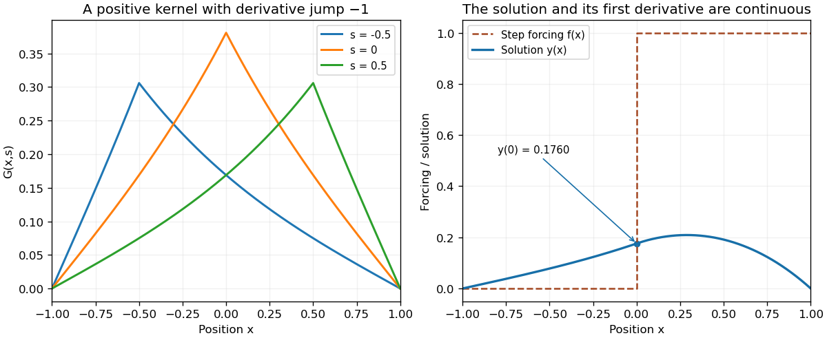
Write the equation as $Ly=f$ with $L=-d^2/d{x}^2+1$. Homogeneous solutions vanishing at the left and right endpoints are $u_L(x)=\sinh (1+x)$ and $u_R(x)=\sinh (1-x)$. Their Wronskian is $u_L{u}_R^{\prime }-u_L^{\prime }{u}_R=-\sinh 2$. The Dirichlet Green kernel for minus second derivative plus one is thereforeIt vanishes at $x=\pm 1$, is continuous at $x=s$, and its first derivative has jump $-1$. Thus $LG(\cdot ,s)={\delta }_s$ in the distributional derivative sense, with the sign appropriate to $L=-d^2/d{x}^2+1$. Integration against $f$ gives the required boundary-value solution. The kernel is positive and symmetric, as is also apparent in the figure.

For the specified step forcing only $0\le s\le 1$ contributes at $x=0$, givingThe discontinuity in $f$ gives a piecewise twice-differentiable solution with continuous value and first derivative, rather than a jump in $y$ itself.

The fundamental theorem of calculus first gives $y^{\prime }(x)=1+{\int }_0^{x}f(y(s))ds$. Integrating again, or differentiating the proposed expression twice and checking its initial values, yields the Volterra integral equationFor $f(y)=-y$, the initial value problem is solved by $\boxed{y(x)=\sin x}$. Its Picard iteration constructs the sine series directly. The base approximation is $y_0(x)=x$. Ifthen elementary integration givesSubstituting this finite sum in the next update, then shifting its index, proves the same formula with $n+1$ in place of $n$. This is the required mathematical induction. The resulting partial sums converge to $\boxed{\sin x}$ for every real $x$, and uniformly on every bounded interval: the absolute terms on $|x|\le R$ are bounded by the convergent series ${\sum }_k{R}^{2k+1}/(2k+1)!$.

The printed update lists $n=1,2,\dots$, which would leave $y_1$ unspecified if read literally. The usual Picard iteration, and the requested induction from $y_0$, use the update starting at $n=0$; that intended convention is used here.