Topics (384k) Articles (398k) Users (410) Discussions (242) Comments (383) Files (13k) New article

An ideal cryptographic functionality is an executable specification of a desired cryptographic service, represented as a trusted computation. Its interfaces specify inputs, outputs, state, permitted cryptographic leakage and permitted adversarial influence. In universal composability, honest-party forwarding interfaces connect it to the cryptographic environment, while the cryptographic simulator uses its adversarial interface.[ref]
Universally Composable Security: A Tutorial by Ran Canetti. PDF pp. 25–27, ideal functionality and its protocol wrapper
An ideal service is a way to state the security goal; it does not assert that the deployed system contains a physically trusted central machine. A cryptographic protocol realizes the service only if the relevant real/ideal comparison is proved.
For a concrete original specification, consider a single-message channel between two fixed, honest parties, with no party corruption in this toy model. Its state begins empty. On the designated sender's submission of , it stores the message under the session label and marks it pending. It reveals the session label, sender, recipient and byte length to the adversarial interface, but not . A later delivery instruction naming that pending session makes it output the stored to the designated recipient and mark the session delivered. Further delivery instructions for that session have no effect; a second submission for the same session is rejected.
This state machine gives both message authentication and message confidentiality specific meanings. The adversarial interface has no instruction for replacing the stored message or impersonating the designated sender. It can delay delivery indefinitely. Thus the toy specification permits length disclosure and denial of delivery, while excluding content disclosure through that interface, message replacement and repeated delivery. These are separate choices, rather than consequences of the word “secure”. The primary tutorial similarly distinguishes authenticated communication, delayed delivery, corruption and message-hiding guarantees.[ref]
Universally Composable Security: A Tutorial by Ran Canetti. PDF pp. 28–33, successive communication functionalities and their exposed information
For an example execution, the sender submits ASCII bytes
41 42 43 under a fresh session label. Before delivery, the simulator learns length three and the endpoints. On the first delivery instruction the recipient receives those three stored bytes. A second delivery instruction produces no new recipient output. If no delivery instruction arrives, the message remains pending. An observed recipient output 41 42 44 would violate this toy specification, regardless of whether it had the correct length.Stating these transitions makes a proof obligation testable: an implementation must match the specified service's observable behavior against every allowed cryptographic environment. Changing the permitted cryptographic leakage, delivery rule or corruption behavior changes the service being implemented.
A cryptographic simulator is an algorithm in a security proof that reproduces an adversary's externally observable behavior using the interfaces and cryptographic leakage allowed by an ideal cryptographic functionality. In universal composability, substituting it for the real adversary should leave every allowed cryptographic environment unable to distinguish real and ideal executions efficiently.[ref]
Universally Composable Security: A Tutorial by Ran Canetti. PDF pp. 23–26, emulation and realization of an ideal functionality
The central question is what information the simulator receives. An original elementary example uses a one-time pad. For a fixed -bit message , let its fresh secret key be uniform on . Its ciphertext is , where is bitwise exclusive or. For every -bit value ,A simulator told only can therefore reproduce this one ciphertext's distribution by generating independent uniform bits, without knowing . With , each of the 32 possible ciphertexts has probability in both constructions. This is a direct distribution calculation, not a complete universal composability proof for a messaging system: other visible inputs, outputs and correlations would also need to match.
Now modify the toy system so its visible packet includes a secret input bit in the clear. Suppose the cryptographic environment selected uniformly and the ideal service reveals neither nor any correlated information before the simulator must report its guessed packet bit . In the real system the environment's test succeeds with probability one. Any simulator whose information is independent of succeeds with probability , even without a computation bound. The cryptographic distinguishing advantage is therefore .
Allowing the ideal service to reveal would remove that particular simulation obstacle, but would specify a different disclosure policy. A valid simulator must use the actual permitted cryptographic leakage, rather than assume access to an honest party's private data.
More generally, reproducing a cryptographic transcript requires its correlations with the cryptographic environment's state to be correct. Sampling plausible-looking individual messages is insufficient. Efficiency also matters: an unbounded reconstruction algorithm does not supply a polynomial time simulator when the security definition requires one.
A cryptographic environment is the interactive external context used to judge a cryptographic protocol in universal composability. It supplies honest parties' inputs, observes their outputs, communicates with the adversary, and ultimately outputs a decision bit. The comparison asks whether this bit's probability distribution changes detectably between the real execution and an ideal execution with a cryptographic simulator.[ref]
Universally Composable Security: A Tutorial by Ran Canetti. PDF pp. 20–24, execution model, protocol emulation and quantitative formulation
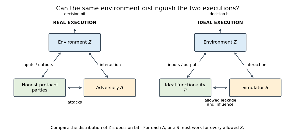
The same cryptographic environment observes either a real protocol and adversary or an ideal service and simulator. Honest-party forwarding is collapsed into the ideal-service box.
Details. The cryptographic environment models other software using the service, including choices depending on earlier outputs. It can retain private information with which to check later responses. Its view therefore includes the relationship between inputs, outputs and adversarial messages, not just isolated packet statistics.
An original two-bit example shows why that relationship matters. Let be a random variable with the uniform distribution on a finite set . One system returns ; another returns with an independent uniform bit. Each individual coordinate has the same marginal distribution in both systems. Nevertheless, the test “accept exactly when the two bits agree” has acceptance probabilitiesIts cryptographic distinguishing advantage is . Matching each output's marginal does not match their joint probability distribution. An interactive cryptographic environment can perform corresponding consistency checks against its retained inputs.
In the computational definition, the cryptographic environment has the specified polynomial time bound indexed by the cryptographic security parameter. For each real adversary, one cryptographic simulator must handle every allowed cryptographic environment; choosing a new simulator after learning which particular context will test it changes the requirement.[ref]
Universally Composable Security: A Tutorial by Ran Canetti. PDF p. 23, quantifier order; pp. 74–76, general formulation and restrictions
This breadth explains the usefulness of universal composability: a service can be analysed within a larger application context. The conclusion still concerns the interactions and cryptographic leakage admitted by the stated execution model.
The kilogram is the SI base unit; prefixes for decimal multiples and submultiples of mass are attached to gram. This special convention gives milligram and microgram, rather than stacked prefixes on kilogram. Mass remains distinct from weight, a force.[ref]
The International System of Units (SI), ninth edition, SI Brochure. §3, prefixes and the kilogram exception
A light-year is the length travelled by light in vacuum during one Julian year of exactly 365.25 days. Using seconds per day and the exact vacuum speed of light givesIt is therefore approximately metres, or 9.46 trillion kilometres. The Julian-year convention matters because a calendar year need not have that duration.[ref]
For a stationary source four light-years away in an idealized flat spacetime, light takes four Julian years to reach the observer. The distance unit and the propagation time remain different physical quantities. In an expanding universe, present distance, lookback time multiplied by the speed of light, and luminosity distance generally differ, so this simple nearby-source interpretation cannot be applied to every cosmological distance.
An inch is a unit of length defined byexactly. Thus an inch is a fixed fraction of the metre, not an independently measured physical constant. The United States announcement of the international conversion made it effective on 1 July 1959.[ref]
A part specified as long therefore has nominal length . If its manufacturing tolerance is , the converted tolerance is . Exact conversion preserves the uncertainty or tolerance already present in the specification; it does not make the manufactured part exact.
For an area, square the conversion: . Multiplying an area by only would fail dimensional analysis. The same distinction matters when converting pixel density, where inches appear in the denominator.
The bending rigidity of an unbonded fibre bundle relates total bending moment to curvature in a stated bending model. If slender material fibres slide longitudinally without appreciable friction, each bends about its own neutral axis. With the same imposed small curvature and no additional axial tension, strand contributes , givingHere is that strand's second moment of area about its own bending axis. The underlying linear elasticity relation is the beam moment-curvature law.[ref] Adding offset-area terms as though all strands shared one neutral axis would impose a different mechanical constraint.
An original two-strand comparison makes the difference quantitative. Take two identical circular strands of radius , with centres vertically separated by , bending in the plane containing their centres. Each has and . In the freely sliding model,For a separate idealization, bond the strands perfectly along their contact so they share a common neutral axis halfway between the centres. Neglect the bond's own area and compliance. Integrating squared distance from that common axis givesFor stipulated and , these are approximately and . At , the corresponding moments are and . Both specimens contain the same strand material; their ability to exchange longitudinal force differs.
A physical comparison would impose end rotations, permit the relative end travel required for inter-fibre sliding, and measure bending moment and curvature. Clamping every strand to identical end displacements, adding axial tension or allowing friction can change the response. The factor five above belongs to this two-strand geometry and ideal bond, not to every bundle. The equal-material subdivision model in material fibre makes a different comparison with a solid circular rod.
The bundle material area fraction is the fraction of a stated bundle envelope occupied by strand material in a specified transverse section:Here includes spaces between material fibres, while excludes them. Count each strand area once and state how the envelope is drawn. A tighter envelope can increase without adding material. For parallel prismatic strands and a constant envelope over common length , the corresponding volumes are and , so the volume fraction equals under those assumptions.
An original two-strand example shows why an average diameter is insufficient. Take circular strand radii and , inside a stipulated envelope of area . ThenReplacing both radii by their arithmetic mean would give and , underestimating the material area by twenty percent. Area depends on the mean squared radius, not merely the square of the mean radius.
For straight, equally strained strands of a common Young's modulus , the axial stiffness is . Dividing the measured rigidity by instead gives the envelope-based effective modulus , rather than the strand material's . This uses the uniform-bar relation applied to parallel strands.[ref]
Structural Stiffness Concept by TU Delft OpenCourseWare. Axial relation and distinction between structural geometry and material properties
A physical estimate can image a transverse section, establish measurement calibration for image lengths, identify the strand boundaries and calculate both areas from the same section. State section orientation: an oblique image is not automatically a perpendicular-area measurement. Distinguish spaces between strands from internal voids within a strand if the intended quantity is solid material area. Changes of envelope convention or classification must not be mistaken for changes in material quantity.
Inter-fibre sliding is relative tangential motion between contacting material fibres. It is distinct from stretching both strands together: equal axial extension can occur with no relative motion at a contact, while bending can require strands to exchange longitudinal position. For local strand displacements and and a contact tangent , the contact slip displacement isThe contact and the sign of must be specified. Contact friction can oppose changing even in an unbonded material-fibre bundle.
An original bending geometry makes the required relative travel visible. Consider two nearby reference paths of radii and , turning through the same angle , measured in radians. Their arc lengths differ byFor chosen separation and turn angle , this mismatch is . If the strands remain inextensible while following those paths, material must feed through the ends to accommodate the difference. Fixing both ends of equal-length strands to remain aligned instead imposes additional strain or a change in the assumed geometry.
This explains the importance of a separate neutral axis for each strand in the freely sliding model for bending rigidity of an unbonded fibre bundle. Bonding imposes longitudinal compatibility and can require axial tension in some strands and compression in others. The usual beam model relates the resulting axial strain to position relative to a common neutral axis.[ref]
A useful mechanical test marks neighbouring strands, bends the assembly while allowing end travel, and measures their relative mark positions. Repeating the bend with constrained ends tests a different loading condition. Record contact loading and bend history: an absence of observed slip at small applied force does not by itself establish a permanent bond.
The TeX line penalty, set by
\linepenalty, enters the per-line base used to calculate typesetting demerits. In the ordinary finite calculation, a line with typesetting badness contributes before breakpoint and neighbour-dependent terms, where denotes the chosen line penalty.[ref]TeX source code by Donald E. Knuth. try_break: line_penalty+b is squared before other contributions
The algebra shows how it affects a candidate with lines:Changing therefore changes both the line-count term and the way spacing costs enter the comparison.
For a chosen example, assume two feasible layouts have badness profiles and , with all other costs zero and values below saturation. At ,At ,The preferred candidate changes. These are illustrative profiles and parameter values. Actual line breaking must also account for feasible endpoints, typesetting penalties and possible line-breaking fitness class changes.
A culture collection maintains documented living cultures of microorganisms for later study and comparison. Its scientific resource consists of both the biological material and the records connecting that material to its origin, identity and measured properties. Microbial culture preservation maintains recoverable material, while microbial culture authentication investigates whether it is the intended strain.[ref]
Guidelines for the Establishment and Operation of Collections of Cultures of Microorganisms by the World Federation for Culture Collections. third edition, February 2010; sections 7, 8 and 11, preservation, authentication and documentation
These functions support reproducibility. A reported effect can be tested on a documented reference rather than on an organism identified only by an informal description. A type strain has an additional nomenclatural role, but a culture collection can also maintain other research strains.[ref]
Guidelines for the Establishment and Operation of Collections of Cultures of Microorganisms by the World Federation for Culture Collections. sections 5 and 8, holdings and accurately identified reference material
Identity and viability are distinct endpoints. In an invented inspection of twenty stored cultures, suppose eighteen yield viable growth and seventeen of those eighteen match the intended identity. The observed recovery fraction is , the matching fraction among recovered cultures is , and the fraction passing both checks is . Reporting just one percentage would conceal which question was tested. These counts illustrate assessment, rather than collection performance data.
ATCC's own account combines morphological, biochemical and genotypic characterization when assessing its prokaryotic materials. Such complementary observations test more than whether a tube produces growth.[ref]
Authentication of Prokaryotes at ATCC by ATCC. Morphology and purity; Biochemical analyses; Genotypic characterization
A culture collection consequently provides a connection between a named biological reference and material that another laboratory can actually examine.Intermittency is the uneven concentration of turbulent fluctuations or dissipation into relatively intense events separated by quieter regions or intervals. It often appears statistically as increasingly non-Gaussian velocity or magnetic-field increments at smaller separations. A turbulent signal can therefore have a moderate average variance while rare events dominate its higher moments.[ref]
Intermittency in the solar wind turbulence through probability distribution functions of fluctuations by Luca Sorriso-Valvo and others. Abstract: scale-dependent non-Gaussian fluctuation distributions and mixtures of variances
One useful diagnostic is the increment flatnessusing the same structure function component and convention in both moments. A centered Gaussian has . Increasing towards small scales indicates increasingly strong relative tails, although measurement noise and nonstationary mixtures also need checking.
A toy distribution isolates the rare-event effect. Let vanish with probability and take values and with probability each. ThenAt , the variance is still but the flatness is . This is an illustrative marginal distribution, not a construction of a complete turbulent field.
Spacecraft measurements provide a concrete application. Analysis of Helios 2 magnetic and velocity records compared increments at different lags and heliocentric distances, finding scale-dependent flatness in both fast and slow solar wind. Mapping time lag to spatial separation requires an advection assumption. Flatness characterizes the fluctuations; by itself it does not establish the sign or magnitude of an energy cascade.[ref]
A structure function measures moments of a field's differences across a separation. For a velocity field , define the longitudinal incrementThe average may be over an ensemble or over a suitable homogeneous sample. Stating the component, separation direction and absolute-value convention matters: signed odd moments contain information that absolute moments erase.[ref]
Dissipation of Energy in the Locally Isotropic Turbulence by Andrei N. Kolmogorov. Opening definitions and longitudinal second/third moments, translated pages 15–16
An independent smooth-field example is in one dimension, averaged over a whole period. Direct integration givesThe quadratic small-separation behavior records differentiability. A constant offset added to the velocity disappears from every increment.
The signed third moment has a special physical role. In the inertial range of high-Reynolds-number, locally isotropic, incompressible turbulence under the usual stationary energy-balance assumptions,with the mean dissipation rate per unit mass. This relation concerns a signed cubic increment, not as defined with an absolute value above. Its sign records a directed transfer that a second-order spectrum cannot determine. At finite viscosity the energy-balance relation has an additional derivative term; anisotropic, transient or compressible data need their own justification before this inertial-range formula is applied.[ref]
Dissipation of Energy in the Locally Isotropic Turbulence by Andrei N. Kolmogorov. Equations relating third moments, viscous derivative term and mean dissipation, translated pages 15–16
A shell model of turbulence replaces a spatially resolved fluid by a sequence of amplitudes associated with progressively smaller length scales. A typical choice assigns a complex velocity amplitude to the wave-number shell , with . Neighboring shells exchange energy through nonlinear couplings, while forcing supplies energy and viscosity damps high wave numbers. The model retains a scale cascade at far lower cost than direct numerical simulation, while discarding most spatial geometry.[ref]
The basic energy bookkeeping is transparent. WriteIf the nonlinear coupling and end conditions satisfy , differentiating givesThe nonlinearity transfers energy between shells without creating its total. Viscous damping becomes faster at larger : an isolated unforced linear mode decays as .
For an illustrative constant-flux estimate, a transfer time gives , hence . Deviations of higher moments from a single scaling rule can then diagnose intermittency. The estimate is dimensional reasoning, not an exact solution. The published improved coupling was designed to reduce spurious shell correlations while preserving useful conservation and scaling properties.[ref]
Improved shell model of turbulence by Victor S. L'vov and others. Abstract and sections I–II, model motivation and scale correlations
A subgrid-scale model represents the influence of unresolved motion on the quantities retained in a large eddy simulation. Its need follows directly from the nonlinear velocity product in the Navier-Stokes equations: averaging a product generally differs from multiplying the averages.
Let a bar denote a spatial averaging filter. With constant mass density , constant kinematic viscosity , and a time-independent translation-invariant filter on an unbounded or periodic domain, filtering the incompressible momentum equation giveswhere repeated indices use the Einstein summation convention, is pressure, and the subgrid-scale stress in this sign convention isThe assumed filter commutes with the displayed derivatives. The definition of is exact; a closure must approximate it using available resolved information.[ref]
A dynamic subgrid-scale eddy viscosity model by Massimo Germano and others (1990). Section2, equations3–7: filtering, filtered momentum and the unresolved stress
For an elementary example, average two equally weighted values of one velocity component, and . The mean is zero but the mean square is , so the corresponding stress component is . A resolved mean alone has lost the information needed to reconstruct that covariance.
The Smagorinsky model closes the deviatoric part with an eddy viscosity:where is the Kronecker delta, is the resolved strain-rate tensor, a dimensionless model coefficient and a characteristic filter width. The isotropic stress can be included in a modified pressure. This strain-dependent viscosity has its historical origin in Joseph Smagorinsky's atmospheric circulation modelling.[ref]
General Circulation Experiments with the Primitive Equations: I. The Basic Experiment by Joseph Smagorinsky. Abstract: lateral exchange coefficient based on horizontal strain and a length scale
[ref]A dynamic subgrid-scale eddy viscosity model by Massimo Germano and others (1990). Introduction, equations1–2: the standard Smagorinsky expression
For an incompressible flow, the model transfers resolved kinetic energy out at the rate per unit massA fixed nonnegative eddy viscosity therefore permits dissipation but excludes local turbulent backscatter. A dynamic subgrid-scale model can instead estimate its coefficient from resolved stresses at two filter levels. This addresses a modelling choice, rather than changing the exact definition of the unresolved stress.[ref]
A dynamic subgrid-scale eddy viscosity model by Massimo Germano and others (1990). Introduction and Section2: backscatter limitations and the dynamic two-filter construction
A large eddy simulation computes the time-dependent large-scale motion of a turbulent flow while representing the influence of unresolved motion through a subgrid-scale model. A spatial averaging filter specifies which information is retained. The distinction concerns spatial resolution, rather than simply replacing a fluctuating flow by its time average.[ref]
For an elementary illustration, take one component of a periodic velocity field,An ideal filter retaining Fourier modes with integer index at most four keeps the first term and removes the second, whose index is ten. The removed term still contributes to products such as . Filtering the nonlinear Navier-Stokes equations consequently introduces a subgrid-scale stress that cannot generally be reconstructed from the retained velocity field alone.
This gives a computational compromise. Direct numerical simulation must resolve the dynamically relevant dissipative motion, whereas a large eddy simulation resolves a chosen coarser field and models its missing influence. Doubling grid counts in all three directions multiplies the cell count by eight, before any additional time-step cost. The filter, numerical discretization and closure must work together; a coarse grid by itself does not certify a useful approximation.
An early concrete demonstration was James W. Deardorff's 1970 calculation of turbulent channel flow using 6720 uniform grid intervals and strain-dependent coefficients for subgrid effects. The paper compared computed statistics with experimental measurements and reported agreement ranging from good to marginal. That comparison tests a particular simulation, rather than establishing that every resolved structure or model is exact.[ref]
A numerical study of three-dimensional turbulent channel flow at large Reynolds numbers by James W. Deardorff. Printed p. 453, abstract: channel geometry, grid intervals, modeled subgrid effects and statistical comparison
Implementations can supply subgrid dissipation in different ways. The Cardinal documentation, for example, describes a spectral filter used to drain energy from the smallest retained wavelengths; that is a particular numerical treatment, not the definition of all large eddy simulation.[ref]
Large Eddy Simulation in the Cardinal documentation. Opening paragraph and modal-filter description
Pinned article: Introduction to the OurBigBook Project
Welcome to the OurBigBook Project! Our goal is to create the perfect publishing platform for STEM subjects, and get university-level students to write the best free STEM tutorials ever.
Everyone is welcome to create an account and play with the site: ourbigbook.com/go/register. We belive that students themselves can write amazing tutorials, but teachers are welcome too. You can write about anything you want, it doesn't have to be STEM or even educational. Silly test content is very welcome and you won't be penalized in any way. Just keep it legal!
Intro to OurBigBook
. Source. We have two killer features:
- topics: topics group articles by different users with the same title, e.g. here is the topic for the "Fundamental Theorem of Calculus" ourbigbook.com/go/topic/fundamental-theorem-of-calculusArticles of different users are sorted by upvote within each article page. This feature is a bit like:
- a Wikipedia where each user can have their own version of each article
- a Q&A website like Stack Overflow, where multiple people can give their views on a given topic, and the best ones are sorted by upvote. Except you don't need to wait for someone to ask first, and any topic goes, no matter how narrow or broad
This feature makes it possible for readers to find better explanations of any topic created by other writers. And it allows writers to create an explanation in a place that readers might actually find it.
Figure 1. Screenshot of the "Derivative" topic page. View it live at: ourbigbook.com/go/topic/derivativeVideo 2. OurBigBook Web topics demo. Source. - local editing: you can store all your personal knowledge base content locally in a plaintext markup format that can be edited locally and published either:This way you can be sure that even if OurBigBook.com were to go down one day (which we have no plans to do as it is quite cheap to host!), your content will still be perfectly readable as a static site.
- to OurBigBook.com to get awesome multi-user features like topics and likes
- as HTML files to a static website, which you can host yourself for free on many external providers like GitHub Pages, and remain in full control

Figure 2. You can publish local OurBigBook lightweight markup files to either OurBigBook.com or as a static website.
Figure 3. Visual Studio Code extension installation.
Figure 5. . You can also edit articles on the Web editor without installing anything locally. Video 3. Edit locally and publish demo. Source. This shows editing OurBigBook Markup and publishing it using the Visual Studio Code extension. 
- Infinitely deep tables of contents:



All our software is open source and hosted at: github.com/ourbigbook/ourbigbook
Further documentation can be found at: docs.ourbigbook.com
Feel free to reach our to us for any help or suggestions: docs.ourbigbook.com/#contact