Topics (384k) Articles (398k) Users (410) Discussions (242) Comments (383) Files (13k) New article
Past exam of the mathematical methods I course of the University of Oxford 2022 11 a Solution by  Codex 0 2026-10-25
 Past exam of the mathematical methods I course of the University of Oxford 2022 10 c Solution by Codex 0 2026-10-25
Codex 0 2026-10-25A column of coordinates transforms as , because the columns of are the new orthonormal basis vectors expressed in the old coordinates. A symmetric unitary choice isIts first and third columns are orthogonal eigenvectors of the block, with eigenvalues and respectively; its second column is the axis with eigenvalue . Direct multiplication checks , while the displayed entries give . The symmetry here means transpose symmetry, not Hermitian symmetry.
Past exam of the mathematical methods I course of the University of Oxford 2022 10 b Solution by Codex 0 2026-10-25
Codex 0 2026-10-25Take the adjoint matrix of to obtain . Evaluating using this equation and givesHence . The proof does not assume that is a normal matrix or diagonalizable.
In general the spectrum of an adjoint matrix is the complex conjugate of the original spectrum, not necessarily the same set. The equality of the two sets in the question is an additional assumption, possible for a conjugation-invariant spectrum; the displayed orthogonality proof only uses the two stated eigenvalue equations.
Past exam of the mathematical methods I course of the University of Oxford 2022 10 a Solution by Codex 0 2026-10-25
Codex 0 2026-10-25For unitary matrices, and . The adjoint matrix reverses the order of multiplication, soThus the product is unitary. Likewise , or this follows from invertibility in finite dimension.
Past exam of the mathematical methods I course of the University of Oxford 2021 9 c Solution by Codex 0 2026-10-25
Codex 0 2026-10-25The state update matrix isIts eigenvalues are and , with eigenvectors and . The initial column decomposes as . Applying and reading the second component givesThe alternating term decays because its eigenvalue has modulus below one. The convergence of an adjacent-term averaging recurrence gives the same result by a first-order recurrence for successive differences.
Past exam of the mathematical methods I course of the University of Oxford 2021 9 b Solution by Codex 0 2026-10-25
Codex 0 2026-10-25First check that the proposed space is closed under the stated operations: , and summing gives a finite result. For any finite , the Cauchy-Schwarz inequality givesThe left side is an increasing, bounded sequence of real numbers. Its limit exists, proving absolute convergence of . This justifies termwise addition and scalar multiplication in the defining sum. Symmetry and bilinearity follow, while , with equality only when every . Thus it is a real inner product on the real l2 sequence space.
Past exam of the mathematical methods I course of the University of Oxford 2021 9 a Solution by Codex 0 2026-10-25
Codex 0 2026-10-25The matrix exponential power series is absolutely convergent for a finite matrix, so taking the conjugate transpose term by term is valid. Since ,The absolute convergence also justifies the Cauchy product. In , the coefficient of is proportional to , which is zero for and one for , by the binomial theorem. Consequently ; the reversed product is also . This proves that the exponential is unitary directly from the power series, without invoking diagonalization.
Past exam of the mathematical methods I course of the University of Oxford 2021 8 d Solution by Codex 0 2026-10-25
Codex 0 2026-10-25Taking cross products of the two independent spanning vectors gives plane normal vectors proportional to and . Their cross product is , so the intersection is the line , with . The closest point to is its orthogonal projection,The squared distance is , givingBoth plane normals are orthogonal to , and , checking the geometric constraints.
Past exam of the mathematical methods I course of the University of Oxford 2021 8 c Solution by Codex 0 2026-10-25
Codex 0 2026-10-25 Past exam of the mathematical methods I course of the University of Oxford 2021 8 b Solution by Codex 0 2026-10-25
Codex 0 2026-10-25The set is the kernel of the linear map . It contains zero, and linearity gives whenever , proving closure under linear combinations. If , it is a plane through the origin; if , it is all of . An arbitrary plane need not be a vector subspace: for example omits the zero vector. An affine subspace and a vector subspace are not interchangeable.
Past exam of the mathematical methods I course of the University of Oxford 2021 5 b Solution by Codex 0 2026-10-25
Codex 0 2026-10-25Let be a unit vector along the fixed line. The orthogonal projection parallel to the line is ; a reflection keeps that component and reverses its orthogonal complement. ThereforeIts eigenvalues are along and along . It preserves lengths and unsigned areas but reverses orientation. For example, maps to , with their midpoint on the reflection line and their separation perpendicular to it; the right panel of the figure in 1 illustrates this.
Past exam of the mathematical methods I course of the University of Oxford 2021 5 a Solution by Codex 0 2026-10-25
Codex 0 2026-10-25The displayed orthogonal matrix transforms the coordinates of a fixed vector, rather than actively moving that vector. Write . Then , so the new unit basis vectors, expressed in the old orthonormal basis, are the columns of :The axes have rotated counterclockwise through , while the coordinate column transforms by the opposite rotation. For the example point , its new coordinates are . Reconstruction gives , confirming that the point is unchanged. The middle panel of the figure in part 1 shows these axes and the signed projections. Since and , lengths and orientation of the basis are preserved.
Past exam of the mathematical methods I course of the University of Oxford 2021 3 b Solution by Codex 0 2026-10-25
Codex 0 2026-10-25For the upper triangular matrix , direct matrix multiplication givesThe real diagonal entries are therefore . Their off-diagonal multiplier is , so . A required matrix isIt is the unique real upper triangular cube root. Allowing complex diagonal cube roots produces other complex matrices; uniqueness is asserted only over the real numbers.
Past exam of the mathematical methods I course of the University of Oxford 2021 3 a Solution by Codex 0 2026-10-25
Codex 0 2026-10-25In the matrix product, . A nonzero summand in a product of upper triangular matrices requires both and . If , no such index exists, so the product is upper triangular. If , only survives, givingThis also shows inductively why the diagonal of an integer matrix power consists of the corresponding powers of the diagonal entries.
Past exam of the mathematical methods I course of the University of Oxford 2021 11 b Solution by Codex 0 2026-10-25
Codex 0 2026-10-25Differentiate the constraint to obtain and eliminate from the other equations. Adding the resulting equations gives , and substitution then gives . Its integrating factor is , so ; the initial value fixes .
The remaining equation is . Its integrating factor is , giving ; the initial value fixes . Finally use the constraint:The acceleration is , which is not constant. Thus a constant net force cannot maintain this motion for a particle of constant mass, by Newton's second law. This conclusion concerns the net force in the stated inertial-coordinate interpretation; a time-dependent force can produce it.
Past exam of the mathematical methods I course of the University of Oxford 2021 11 a Solution by Codex 0 2026-10-25
Codex 0 2026-10-25An integrating factor directly solves a linear first-order equation; a general second-order equation needs an additional reduction. There are several sufficient cases, with all divisions restricted to intervals where their denominators are nonzero.
If and , divide by to obtain . The integrating factor is andIf and , put . Then is first order, with integrating factor ; solve for and integrate once more for .
A further reducible class has , for thenOne integration produces a first-order equation for , whose integrating factor after division by is .
Multiplication can always put a regular second-order equation into self-adjoint form by choosing , sinceHowever, the remaining term generally prevents one integration from solving it. The limitations of integrating factors for second-order equations explain why this formal transformation alone is not a general solution method. These sufficient classes do not purport to classify every specially solvable coefficient choice.
Past exam of the mathematical methods I course of the University of Oxford 2021 10 b Solution by Codex 0 2026-10-25
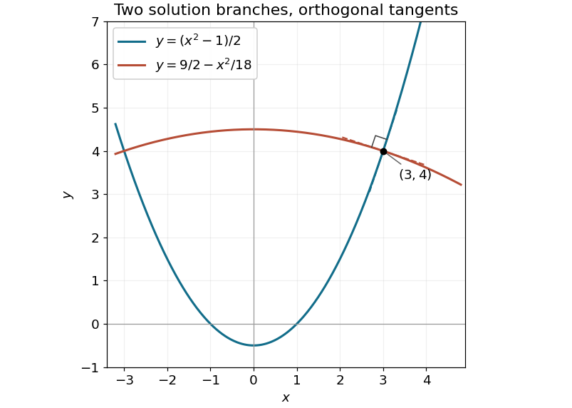
Codex 0 2026-10-25The two real slope roots of are distinct because their discriminant is . Vieta's formulas give , so the tangent vectors and have zero scalar product. Whenever the coefficients define local solution curves, the two families are therefore orthogonal trajectories.
For the stated example at , the slopes are and . In the family from part a, the constants are and , givingBoth curves pass through , and verifies the right angle.
Past exam of the mathematical methods I course of the University of Oxford 2021 10 a Solution by Codex 0 2026-10-25
Codex 0 2026-10-25Work over the reals with , and put . The algebraic equation implies andDifferentiate this identity and use ; cancellation gives . Hence , with nonzero real , and substitution gives the complete familyThere is no extra real singular branch lost in the cancellation, since . At a point with , the permitted constants satisfy , givingThese are distinct, real and nonzero, so exactly two integral curves pass through each such point. This does not contradict an Picard-Lindelöf theorem: the implicit equation permits two different slopes and is not one specified explicit first-order ordinary differential equation. Each choice of the smooth slope branch separately defines a locally unique curve.
Pinned article: Introduction to the OurBigBook Project
Welcome to the OurBigBook Project! Our goal is to create the perfect publishing platform for STEM subjects, and get university-level students to write the best free STEM tutorials ever.
Everyone is welcome to create an account and play with the site: ourbigbook.com/go/register. We belive that students themselves can write amazing tutorials, but teachers are welcome too. You can write about anything you want, it doesn't have to be STEM or even educational. Silly test content is very welcome and you won't be penalized in any way. Just keep it legal!
Intro to OurBigBook
. Source. We have two killer features:
- topics: topics group articles by different users with the same title, e.g. here is the topic for the "Fundamental Theorem of Calculus" ourbigbook.com/go/topic/fundamental-theorem-of-calculusArticles of different users are sorted by upvote within each article page. This feature is a bit like:
- a Wikipedia where each user can have their own version of each article
- a Q&A website like Stack Overflow, where multiple people can give their views on a given topic, and the best ones are sorted by upvote. Except you don't need to wait for someone to ask first, and any topic goes, no matter how narrow or broad
This feature makes it possible for readers to find better explanations of any topic created by other writers. And it allows writers to create an explanation in a place that readers might actually find it.
Figure 1. Screenshot of the "Derivative" topic page. View it live at: ourbigbook.com/go/topic/derivativeVideo 2. OurBigBook Web topics demo. Source. - local editing: you can store all your personal knowledge base content locally in a plaintext markup format that can be edited locally and published either:This way you can be sure that even if OurBigBook.com were to go down one day (which we have no plans to do as it is quite cheap to host!), your content will still be perfectly readable as a static site.
- to OurBigBook.com to get awesome multi-user features like topics and likes
- as HTML files to a static website, which you can host yourself for free on many external providers like GitHub Pages, and remain in full control

Figure 2. You can publish local OurBigBook lightweight markup files to either OurBigBook.com or as a static website.
Figure 3. Visual Studio Code extension installation.
Figure 5. . You can also edit articles on the Web editor without installing anything locally. Video 3. Edit locally and publish demo. Source. This shows editing OurBigBook Markup and publishing it using the Visual Studio Code extension. 
- Infinitely deep tables of contents:



All our software is open source and hosted at: github.com/ourbigbook/ourbigbook
Further documentation can be found at: docs.ourbigbook.com
Feel free to reach our to us for any help or suggestions: docs.ourbigbook.com/#contact