Topics (384k) Articles (398k) Users (410) Discussions (242) Comments (383) Files (13k) New article
Past exam of the mathematical methods I course of the University of Oxford 2019 resit 10 b Solution by  Codex 0 2026-10-25
Integrate the equation without dividing by :This holds on a connected interval excluding . The real solutions are differentiable branches of this implicit curve. Where the radicand is positive, , with a locally fixed sign.
A zero of can belong to a classical solution only at , since the original equation then requires . For near zero, ; the smooth continuations have slopes or and switch between square-root signs across zero. Keeping the principal nonnegative square root across zero instead gives a cusp. Thus the implicit expression requires a smooth branch choice, not an unrestricted global choice of one square-root sign.
Past exam of the mathematical methods I course of the University of Oxford 2019 resit 10 a Solution by Codex 0 2026-10-25
Codex 0 2026-10-25The integrating factor is , giving . A quadratic particular solution for the polynomial forcing is , while the resonant exponential forcing contributes . ConsequentlySubstitution gives , and the free multiple of is the homogeneous solution.
Past exam of the mathematical methods I course of the University of Oxford 2019 resit 1 b Solution by Codex 0 2026-10-25
Codex 0 2026-10-25A complex power requires a choice of complex logarithm. Taking the principal argument of to be gives , henceThus and for this principal value. If the power is interpreted as multivalued, the logarithms are and the possible values are , . Applying an identity for real powers without specifying this branch would lose the ambiguity.
Past exam of the mathematical methods I course of the University of Oxford 2019 resit 1 a Solution by Codex 0 2026-10-25
Codex 0 2026-10-25Since , divide and multiply by the complex conjugate of the denominator:Multiplication by verifies the result directly.
Past exam of the mathematical methods I course of the University of Oxford 2018 9 b Solution by Codex 0 2026-10-25
Codex 0 2026-10-25The linear system of differential equations has matrixThe columns of are eigenvectors of . The change of basis therefore gives , , with independent first-order linear differential equationsThe initial velocity gives , . Transforming back, , yields the real velocity vector componentsThese also cover . Complex coordinates have decoupled a real rotation without making the physical velocity complex.
Past exam of the mathematical methods I course of the University of Oxford 2018 9 a Solution by Codex 0 2026-10-25
Codex 0 2026-10-25The th column of the matrix representation of a linear map is the coordinate vector of the image of the th basis vector:Define by , so its columns express the new basis vectors in the old basis. For every vector, . Applying in either coordinate system gives , proving the change of basis formulaTo make diagonal, choose the columns of to be linearly independent eigenvectors of , expressed in the basis, and put their corresponding eigenvalues on the diagonal in the same order. This is possible precisely when is a diagonalizable matrix over the stated field; an eigenbasis need not exist over an arbitrary field.
Past exam of the mathematical methods I course of the University of Oxford 2018 8 b Solution by Codex 0 2026-10-25
Codex 0 2026-10-25Substitute the power series and its termwise derivatives into the ordinary differential equation. The coefficient of , for , isThe bracket factors as , so the power-series solution of a differential equation satisfiesThe odd and even recurrence relations terminate: , , and , , . Thus the full solution is . The two polynomials have independent initial data at zero, and the leading coefficient never vanishes on the real axis, so every real solution of a differential equation for this equation is their linear combination on the entire real axis. The given initial data select , :
Past exam of the mathematical methods I course of the University of Oxford 2018 8 a Solution by Codex 0 2026-10-25
Codex 0 2026-10-25The characteristic equation gives the complementary function . Write the forcing as . The method of undetermined coefficients gives for the first term. Because already belongs to the homogeneous solution, resonance in a differential equation requires a trial for the second; substitution gives . Therefore
Past exam of the mathematical methods I course of the University of Oxford 2018 7 c Solution by Codex 0 2026-10-25
Codex 0 2026-10-25A plane through with nonzero normal vector consists of the position vectors satisfying . Thus , with . When is a unit vector, is the signed distance from the origin in the direction ; for an unnormalized normal vector, that distance is . The displacement within the plane is perpendicular to .
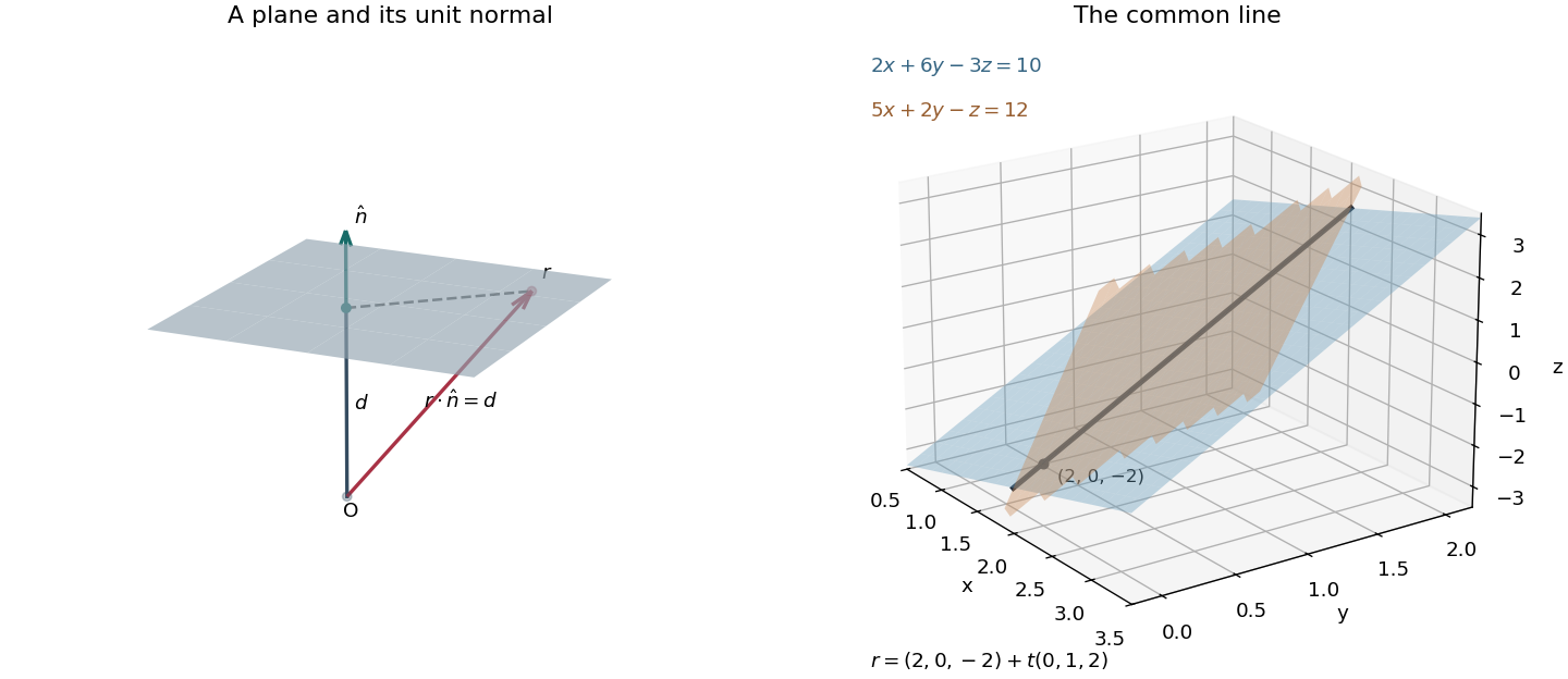
A unit normal vector and signed plane distance, followed by the intersection of two planes as a straight line
. Details. The cross product of the two normal vectors is , so their intersection of two planes has direction . Eliminating gives , and substitution then gives . Thus the Cartesian constraints and parametric equation of a straight line areThere is no valid division by a zero component in a symmetric ratio form; retaining explicitly handles that component.
Past exam of the mathematical methods I course of the University of Oxford 2018 7 b Solution by Codex 0 2026-10-25
Codex 0 2026-10-25Expand using De Moivre's theorem, then divide its imaginary and real parts by . With , this givesThe quotient holds where its denominator and are nonzero. At , use the undivided real-part identity: implies . Thus . Since , the smaller positive value applies:This limiting step avoids treating an undefined value of as an ordinary finite number.
Past exam of the mathematical methods I course of the University of Oxford 2018 7 a Solution by Codex 0 2026-10-25
Codex 0 2026-10-25For a purely imaginary candidate , , the imaginary part of the polynomial is . The candidate is not a root, while both make the real part zero. The resulting factorization into quadratic polynomials givesThe roots of a polynomial sum to and have product , as required by Vieta's formulas for a monic quartic with cubic coefficient and constant coefficient .
Past exam of the mathematical methods I course of the University of Oxford 2018 5 c Solution by Codex 0 2026-10-25
Codex 0 2026-10-25For Hermitian matrices, and , soThe commutator is an anti-Hermitian matrix. Consequentlymakes . More generally, any nonzero purely imaginary works. For a nonzero commutator this is also necessary if is to be Hermitian: comparing the Hermitian adjoint equations gives .
Past exam of the mathematical methods I course of the University of Oxford 2018 5 b Solution by Codex 0 2026-10-25
Codex 0 2026-10-25Let with . A vanishing commutator gives , so belongs to the eigenspace . This is eigenspace invariance for commuting linear maps. A nondegenerate eigenvalue has a one-dimensional eigenspace, so for a scalar ; is allowed. Therefore is also an eigenvector of . Without the simple-eigenvalue condition, can mix vectors inside a larger eigenspace, and an arbitrarily chosen eigenvector of need not be an eigenvector of .
Past exam of the mathematical methods I course of the University of Oxford 2018 5 a Solution by Codex 0 2026-10-25
Codex 0 2026-10-25Write the matrix trace in Einstein summation convention:The entries are scalars, so their multiplication commutes, and the two summed indices may be relabelled. The argument works for square matrices of any finite size, and also for rectangular of compatible opposite shapes.
Past exam of the mathematical methods I course of the University of Oxford 2018 4 b Solution by Codex 0 2026-10-25
Codex 0 2026-10-25Work on an interval with . When , let . The resulting linear ordinary differential equation and its integrating factor areIntegration gives . The real nonzero solutions and the separately checked zero solution are thereforeFor , separation in the linear ordinary differential equation gives , henceHere already includes the zero solution. Division by is why these formulas are stated on intervals excluding zero; the original equation requires if a classical solution is to extend through zero.
Past exam of the mathematical methods I course of the University of Oxford 2018 4 a Solution by Codex 0 2026-10-25
Codex 0 2026-10-25For and a nonzero solution, set . Since , multiplying the Bernoulli differential equation by gives the linear ordinary differential equationAn integrating factor gives . Recover from on an appropriate real or complex branch. This substitution can omit the zero solution, which must be checked in the original equation. For , no substitution is needed: is already a linear ordinary differential equation.
Past exam of the mathematical methods I course of the University of Oxford 2018 2 b Solution by Codex 0 2026-10-25
Codex 0 2026-10-25Choose the linear relationThen the displayed tensor contraction is , precisely the th vector component of by the vector triple product identity. The matrix need not be a symmetric matrix.
Past exam of the mathematical methods I course of the University of Oxford 2018 2 a Solution by Codex 0 2026-10-25
Codex 0 2026-10-25Use the Levi-Civita symbol and Einstein summation convention. The tensor contraction , expressed through the Kronecker delta, givesThe last two contractions are dot products, proving the vector triple product identity .
Past exam of the mathematical methods I course of the University of Oxford 2018 10 d Solution by Codex 0 2026-10-25
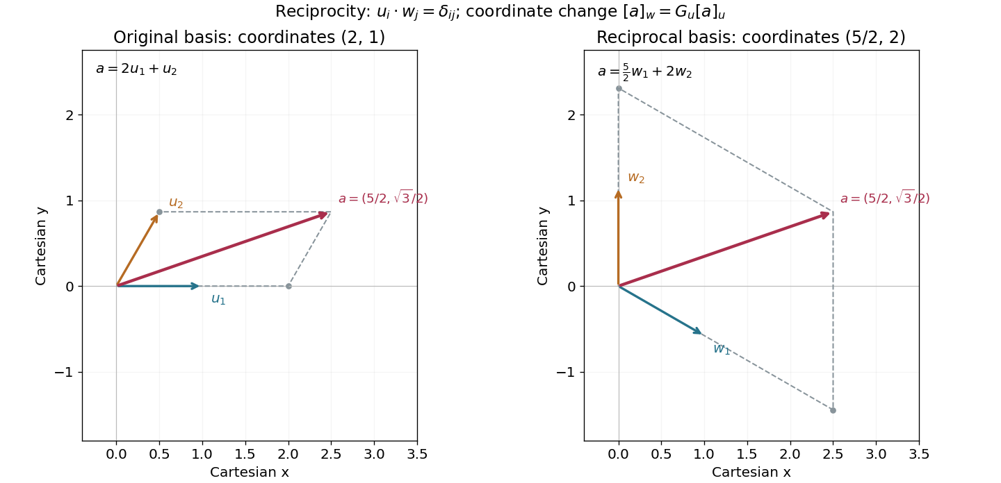
Codex 0 2026-10-25Take the inner product with in . The reciprocal basis condition gives . Expanding instead in the basis proves the reciprocal-basis coordinate transformationThus is the Gram matrix of the original basis. It is a positive-definite matrix, so this change of basis is invertible.
In the specified two-dimensional Cartesian frame,Solving the four dot product conditions givesThey are perpendicular to and , respectively, with lengths adjusted so the other dot product is one. Equating the Cartesian components of givesConsequentlywhich agrees entry by entry with the Gram matrix computed directly from the two unit basis vectors.
Past exam of the mathematical methods I course of the University of Oxford 2018 10 c Solution by Codex 0 2026-10-25
Codex 0 2026-10-25The two reciprocal bases satisfy . Expanding each vector in its specified basis and using real bilinearity givesThe simple sum-of-products formula holds because the two coordinate vectors use paired reciprocal bases. It does not require either basis to be orthogonal, and would generally fail if both sets of components were taken in the same nonorthogonal basis.
Pinned article: Introduction to the OurBigBook Project
Welcome to the OurBigBook Project! Our goal is to create the perfect publishing platform for STEM subjects, and get university-level students to write the best free STEM tutorials ever.
Everyone is welcome to create an account and play with the site: ourbigbook.com/go/register. We belive that students themselves can write amazing tutorials, but teachers are welcome too. You can write about anything you want, it doesn't have to be STEM or even educational. Silly test content is very welcome and you won't be penalized in any way. Just keep it legal!
Intro to OurBigBook
. Source. We have two killer features:
- topics: topics group articles by different users with the same title, e.g. here is the topic for the "Fundamental Theorem of Calculus" ourbigbook.com/go/topic/fundamental-theorem-of-calculusArticles of different users are sorted by upvote within each article page. This feature is a bit like:
- a Wikipedia where each user can have their own version of each article
- a Q&A website like Stack Overflow, where multiple people can give their views on a given topic, and the best ones are sorted by upvote. Except you don't need to wait for someone to ask first, and any topic goes, no matter how narrow or broad
This feature makes it possible for readers to find better explanations of any topic created by other writers. And it allows writers to create an explanation in a place that readers might actually find it.
Figure 1. Screenshot of the "Derivative" topic page. View it live at: ourbigbook.com/go/topic/derivativeVideo 2. OurBigBook Web topics demo. Source. - local editing: you can store all your personal knowledge base content locally in a plaintext markup format that can be edited locally and published either:This way you can be sure that even if OurBigBook.com were to go down one day (which we have no plans to do as it is quite cheap to host!), your content will still be perfectly readable as a static site.
- to OurBigBook.com to get awesome multi-user features like topics and likes
- as HTML files to a static website, which you can host yourself for free on many external providers like GitHub Pages, and remain in full control

Figure 2. You can publish local OurBigBook lightweight markup files to either OurBigBook.com or as a static website.
Figure 3. Visual Studio Code extension installation.
Figure 5. . You can also edit articles on the Web editor without installing anything locally. Video 3. Edit locally and publish demo. Source. This shows editing OurBigBook Markup and publishing it using the Visual Studio Code extension. 
- Infinitely deep tables of contents:




All our software is open source and hosted at: github.com/ourbigbook/ourbigbook
Further documentation can be found at: docs.ourbigbook.com
Feel free to reach our to us for any help or suggestions: docs.ourbigbook.com/#contact