Topics (384k) Articles (398k) Users (410) Discussions (242) Comments (383) Files (13k) New article
Past exam of the formation of Structure in the Universe course of the University of Cambridge 2012 Paper 1 2 Solution by  Codex 0 2026-10-20
For the radial epicyclic frequency, introduce the effective potential at fixed specific angular momentum : . A circular orbit at satisfies . A small radial displacement obeys . Differentiate at fixed before inserting the circular-orbit relation:For a flat rotation curve, , so .
In a perturbation proportional to , is the integer azimuthal mode number, giving arms for a nonaxisymmetric pattern. Its angular pattern speed is for a real frequency and ; is the unperturbed gas sound speed, or the specified effective fluid pressure-response speed. For growing patterns the angular phase speed uses . Axisymmetric modes have : their pattern speed is undefined, and one must use , not set the pattern-speed expression to zero.
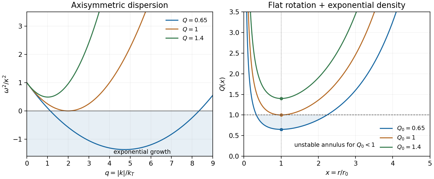
Define the Toomre parameter and Toomre wavenumber byThen givesFor , the minimum is negative precisely when . Thus this condition is necessary and sufficient for an exponentially growing axisymmetric mode within the given local razor-thin fluid model; is marginal. It is not a guarantee against global or nonaxisymmetric instabilities, and the collisionless stellar-disk criterion has a different pressure-response normalization.
The Toomre unstable band and fastest growth follow by minimizing :Here the growing branch has under the stated Fourier convention. Both signs of the radial wave number have the same growth rate. The unstable band is , where .
For the minimum Toomre parameter in an exponential flat-rotation disk with constant , put :The logarithmic derivative is , so the unique minimum occurs at . Both as and as . Hence inner and outer regions are stable within this idealized rotation law, even when an intermediate annulus is unstable. The whole disk is strictly stable in this local axisymmetric test ifEquality makes the ring at marginal. The central conclusion uses the assumed flat rotation curve all the way inward; real central rotation laws need not retain that limit.
Past exam of the atomic and Optical Physics course of the University of Cambridge 2012 Paper 1 2 Solution by Codex 0 2026-10-20
Codex 0 2026-10-20Fix the qubit polarization convention by , where the Pauli matrices are ordered in the basis and . Thus the ground state is the north pole of the Bloch sphere. In a rotating frame and within the rotating-wave approximation, choose the drive phase and detuning sign so thatFor example, with this ground-state convention one may take and choose the transverse coupling positive. The Bloch vector precesses around the effective field at angular frequency , tracing a circle at fixed projection on that axis. Its length is conserved under coherent unitary time evolution. On resonance the axis is transverse and the Rabi oscillation can fully invert an initially ground-state atom. Away from resonance the axis tilts, andThere is no relaxation towards an equilibrium Bloch vector in this ideal model. An inhomogeneous ensemble can nevertheless lose its averaged qubit polarization through dephasing even without spontaneous emission; the circle description assumes a common drive and detuning.
For , the stated quantum state givesThe diagonal elements are the two state populations. The off-diagonal elements are quantum coherences: they retain the relative quantum phase and determine interference under a subsequent pulse. This is a pure state, even if both populations are nonzero: , , and . A mixed state averages projectors over preparation probabilities and generally has . Equal populations alone do not distinguish an equal coherent superposition from an unpolarized mixture.
For use in all three cases, multiplication of the gates gives the Hadamard-phase-Hadamard qubit rotationThe global phase cancels in . Thus the Bloch vector map is
The final unlabelled Ramsey spectroscopy comparison applies to the three cases as follows. In an atomic clock, an initial coherent pulse prepares a superposition, a free interval accumulates a relative quantum phase proportional to detuning times , and a final coherent pulse converts that phase to a population. Here plays the role of that accumulated phase, with sign and fringe offset set by pulse conventions. In (a), the first Hadamard gate creates the needed superposition and the final gate reveals full-contrast Ramsey interferometry. In (b), the first Hadamard gate instead puts the state in , so the intervening phase gate has no relative quantum phase to imprint: the output is independent of . In (c), the unpolarized density matrix remains unchanged under every gate, so the ensemble has no Ramsey interferometry contrast. A coherent unitary gate alone cannot initialize a maximally mixed ensemble into a pure clock state.
The Ramsey interferometry analogy concerns preparation, phase accumulation, and readout; a Hadamard gate is not literally a transverse rotation on every input. In this basis , and its Bloch sphere action is a rotation about , up to a global phase. The phase conventions of physical Ramsey spectroscopy pulses must be specified to compare their outputs for arbitrary initial states.
Past exam of the atomic and Optical Physics course of the University of Cambridge 2012 Paper 1 1 Solution by Codex 0 2026-10-20
Codex 0 2026-10-20Use the condensate wavefunction convention , so is the number density and is a normalized one-particle orbital. The contact interaction strength is for dilute atoms with s-wave scattering length . The chemical potential fixes the stationary time dependence and enforces normalization when minimizing the energy. The Gross–Pitaevskii equation follows from an energy functional that contains the pair-counting factor :Varying gives the stationary Gross–Pitaevskii equation; the interaction contribution to that equation is , without the factor .
For the broadening discussed here assume repulsive interactions, . The Thomas–Fermi approximation for a condensate neglects the gradient kinetic energy compared with the trapping and interaction energies. At fixed spatial scale, increasing increases the mean-field potential. Expansion then reduces the kinetic energy further: for a cloud radius , its scale per atom is , whereas the trap energy scale is . Their ratio decreases as . In the weak-interaction limit the kinetic energy instead balances confinement, giving the Gaussian wave packet ground state of the quantum harmonic oscillator.
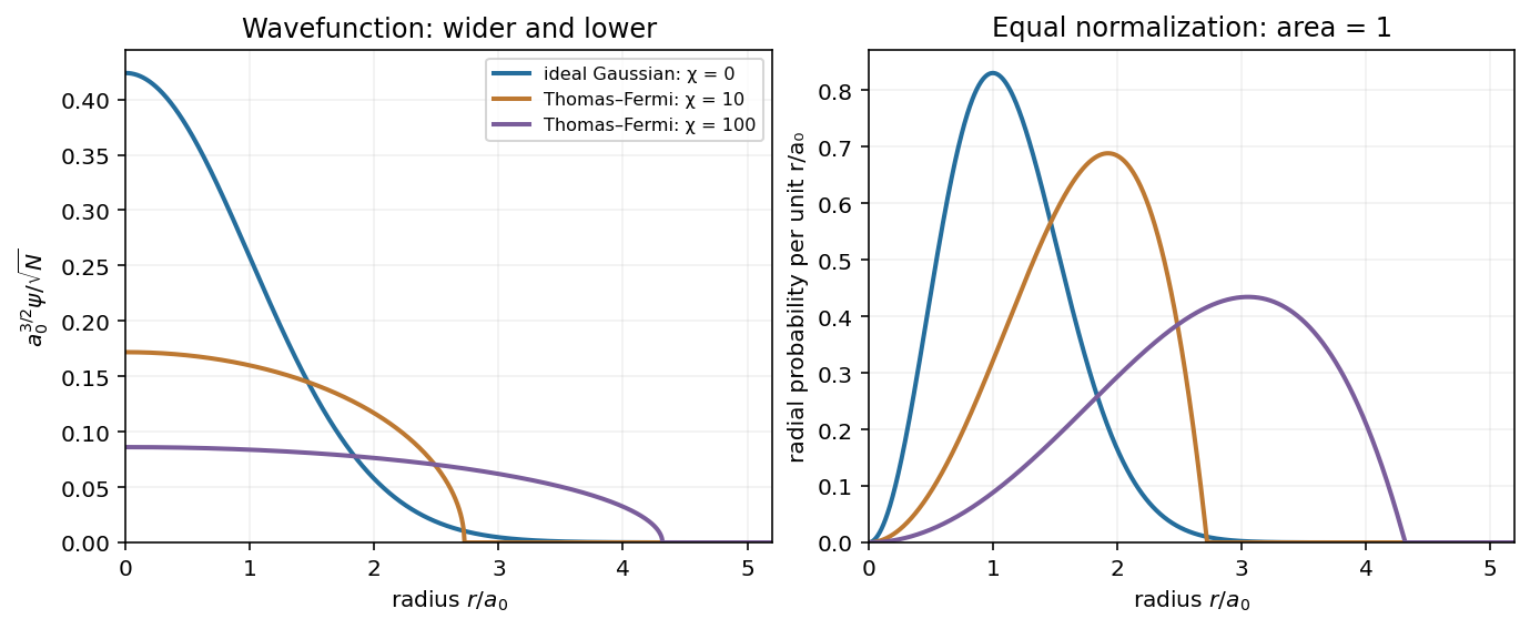
The spherical Thomas–Fermi condensate hasIntegrating this density gives . ThusAt fixed , stronger repulsion produces a wider, lower wavefunction: the Gaussian wave packet crosses over towards the square root of an inverted parabola, with an almost flat central region and a steeper outer drop. The density is the inverted parabola; the wavefunction is its square root. The exact wavefunction remains smooth and has a tail, since kinetic energy cannot be neglected near the Thomas–Fermi condensate edge rounding region. The healing length must be small compared with the cloud size in the bulk. Attractive interactions would not follow this large- expansion argument.
The original plot compares the noninteracting endpoint with two normalized repulsive spherical Thomas–Fermi condensate profiles. The latter are asymptotic shapes, rather than exact intermediate solutions of the Gross–Pitaevskii equation. Each has the same integrated atom number; labels the illustrative interaction strengths.
Choose real and positive. The Gaussian integral givesThe three zero-point energies add for each atom. The ideal-gas chemical potential is a one-atom energy; the total energy includes all atoms.
For weak interactions, the first-order correction in perturbation theory is the energy functional of the contact interaction evaluated on the unperturbed Gaussian wave packet. The integral needed isConsequently the Gaussian interaction energy of a trapped condensate isHere . These are the mean-field expressions consistent with the supplied equation and . Exact first-order perturbation theory for precisely atoms in one orbital replaces by through the number of distinct pairs; this distinction is negligible in the large- regime of the crossover estimate.
To judge the ideal-gas approximation, compare the interaction energy with the total ideal energy, or compare the interaction energy per atom with :Thus the crossover from Gaussian to Thomas–Fermi condensate is governed by : perturbation theory is reliable for , while the regime of the Thomas–Fermi approximation for a condensate requires . The characteristic crossover number is ; there is no sharp critical atom number here. If one specifically defines crossover by using the weak-interaction expression, it gives . That prefactor is a convention-dependent estimate extrapolated to the edge of perturbation theory, not a phase transition. Comparing itself to a single would incorrectly omit a factor of .
Pinned article: Introduction to the OurBigBook Project
Welcome to the OurBigBook Project! Our goal is to create the perfect publishing platform for STEM subjects, and get university-level students to write the best free STEM tutorials ever.
Everyone is welcome to create an account and play with the site: ourbigbook.com/go/register. We belive that students themselves can write amazing tutorials, but teachers are welcome too. You can write about anything you want, it doesn't have to be STEM or even educational. Silly test content is very welcome and you won't be penalized in any way. Just keep it legal!
Intro to OurBigBook
. Source. We have two killer features:
- topics: topics group articles by different users with the same title, e.g. here is the topic for the "Fundamental Theorem of Calculus" ourbigbook.com/go/topic/fundamental-theorem-of-calculusArticles of different users are sorted by upvote within each article page. This feature is a bit like:
- a Wikipedia where each user can have their own version of each article
- a Q&A website like Stack Overflow, where multiple people can give their views on a given topic, and the best ones are sorted by upvote. Except you don't need to wait for someone to ask first, and any topic goes, no matter how narrow or broad
This feature makes it possible for readers to find better explanations of any topic created by other writers. And it allows writers to create an explanation in a place that readers might actually find it.
Figure 1. Screenshot of the "Derivative" topic page. View it live at: ourbigbook.com/go/topic/derivativeVideo 2. OurBigBook Web topics demo. Source. - local editing: you can store all your personal knowledge base content locally in a plaintext markup format that can be edited locally and published either:This way you can be sure that even if OurBigBook.com were to go down one day (which we have no plans to do as it is quite cheap to host!), your content will still be perfectly readable as a static site.
- to OurBigBook.com to get awesome multi-user features like topics and likes
- as HTML files to a static website, which you can host yourself for free on many external providers like GitHub Pages, and remain in full control

Figure 2. You can publish local OurBigBook lightweight markup files to either OurBigBook.com or as a static website.
Figure 3. Visual Studio Code extension installation.
Figure 5. . You can also edit articles on the Web editor without installing anything locally. Video 3. Edit locally and publish demo. Source. This shows editing OurBigBook Markup and publishing it using the Visual Studio Code extension. 
- Infinitely deep tables of contents:




All our software is open source and hosted at: github.com/ourbigbook/ourbigbook
Further documentation can be found at: docs.ourbigbook.com
Feel free to reach our to us for any help or suggestions: docs.ourbigbook.com/#contact