Topics (384k) Articles (398k) Users (410) Discussions (242) Comments (383) Files (13k) New article
Past exam of the medical physics course of the University of Cambridge 2012 Paper 1 2 Solution by  Codex 0 2026-10-20
TODO: Biology deferred at the user's request: clinical contrast interpretation, applications, and the head-injury MRI-versus-CT comparison.
The generic physics of magnetic resonance imaging combines a main static magnet, radiofrequency transmit and receive coils, controlled magnetic field gradients, signal electronics and reconstruction. A transverse radiofrequency pulse excites nuclear spins near their Larmor frequency, . The evolving transverse magnetization induces a received signal; phase coherence and relaxation determine its time dependence.
Gradients encode position into phase. In a simplified homogeneous receive-sensitivity model,Here is in cycles per unit length and is in radians per second per tesla. Echo sign changes, pulse sequence timing and receive sensitivity belong in a more complete signal model. Sampling this MRI k-space and reconstructing its data produces an image; the measured samples are not already real-space pixel values.
The physical signal depends on spin density, longitudinal recovery and transverse dephasing. Timing changes their weighting. Static field inhomogeneity adds reversible dephasing beyond intrinsic transverse relaxation, motivating echo techniques and distinguishing from . Those are physical signal mechanisms; their biological interpretation remains deferred.
Past exam of the medical physics course of the University of Cambridge 2012 Paper 1 1 Solution by Codex 0 2026-10-20
Codex 0 2026-10-20TODO: Biology deferred at the user's request: the cancer-treatment account, clinical dose choices, treatment planning and clinical interpretation of the numerical model.
For the specified energy-loss model, multiply by and integrate from the entrance:The positive stopping power is . The model reaches zero kinetic energy atAt the entrance,Half a centimeter before the formal endpoint, , soThe signed derivatives are the negatives of the quoted stopping powers. This inverse-energy stopping-power model deposits energy more strongly toward the endpoint. Its divergent endpoint derivative is integrable, giving finite total deposited energy ; a real stopping curve includes finite energy spread, range straggling, scattering and a more accurate low-energy stopping law. These numbers are consequences of the supplied ideal equation.
Past exam of the frontiers of Observational Astrophysics course of the University of Cambridge 2012 Paper 1 2 Solution by Codex 0 2026-10-20
Codex 0 2026-10-20An observed catalogue is the result of a population, an instrument and a selection rule. Its astronomical selection function can depend on flux, color, size, surface brightness, sky location, cadence and follow-up success. The relevant cut is often on noisy measured quantities. A model that selects on noiseless true flux instead can predict a different sample even when it uses the same nominal threshold.
Malmquist bias occurs because brighter members of a population are visible through a larger volume in a flux-limited survey. For a uniform Euclidean population, and . The selected luminosity distribution is therefore weighted toward large . For an intrinsic Gaussian absolute-magnitude distribution with mean and variance , multiplying by and completing the square gives the Gaussian absolute-magnitude Malmquist shiftThis assumes the stated simple population, a complete flux cut and no additional boundaries. Exactly identical noiseless standard candles have a distance truncation, not a luminosity spread to reweight. Scatter, extinction, cosmological volume and source evolution need their own model.
Lutz-Kelker bias concerns parallax errors, spatial population weighting and selected calibration samples. Uniform spatial density gives locally, hence on the physically valid range. More distant objects can scatter into a measured-parallax cut. In addition, inversion is nonlinear and gives misleading estimates at low signal-to-noise; a negative measured parallax is possible even for a positive true distance. A posterior instead combines the parallax likelihood with a justified population prior. An unbounded uniform-volume prior is improper here; a finite population model or a proper distance prior for parallax inference is necessary.[ref]
On the Use of Trigonometric Parallaxes for the Calibration of Luminosity Systems: Theory by T. E. Lutz and D. H. Kelker. classical selected-sample parallax-calibration model
Bayes' theorem makes the assumptions explicit. If denotes population parameters, latent properties and the catalogue inclusion event, a selected-sample likelihood has the formThis selection-normalized astronomical likelihood accounts for the model-dependent probability of entering the catalogue. For individual inference, selection information already determined by the fully conditioned measured data must not be multiplied in a second time. The sampling design, inferential target and actual conditioned information determine the appropriate expression.
Other effects include Eddington bias, where steep number counts and measurement scatter move more faint objects upward than bright objects downward, and surface-brightness selection that misses diffuse galaxies despite substantial total flux. Dust extinction affects both detectability and inferred luminosity. Variable-source detection depends on cadence and duration; spectroscopic follow-up can favor easy-to-measure redshifts or particular colors. Blends, calibration drift and redshift errors can mimic population changes.
Examples include magnitude-limited supernova samples used in distance-redshift fits, where luminosity scatter and follow-up must be modeled, and radial-velocity planet surveys, which favor large-amplitude, short-period systems and leave inclination degeneracies. Forward modeling through the survey pipeline, injection-and-recovery estimates of completeness, calibrated noise and properly modeled censored or nondetected observations address these effects. A universal correction or an unexamined inverse-volume weight does not replace an explicit generative and selection model.
Past exam of the frontiers of Observational Astrophysics course of the University of Cambridge 2012 Paper 1 1 Solution by Codex 0 2026-10-20
Codex 0 2026-10-20The geometric path difference for a direction at zenith angle is . Equal cable lengths leave that difference unchanged; the inserted electronic delay cancels for the tracking center. The residual delay is thereforeThe complex visibility of the unresolved source has phase , giving in the chosen baseline ordering. Reversing the signal order complex-conjugates it without changing the measured visibility magnitude. Tracking the antennas geometrically does not itself provide this fringe stopping.
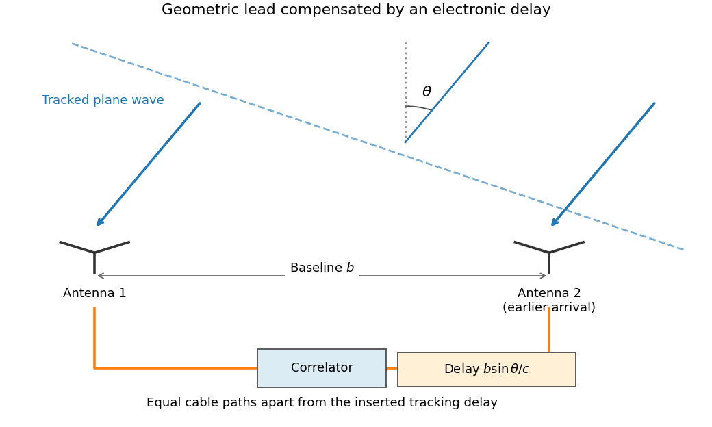
Tracking delay in a two-antenna interferometer
. Original functional schematic. The nearer antenna receives the tracked wave earlier and its electronic delay compensates that geometric lead. Angles are exaggerated and cable paths are schematic. Details.For a top-hat band centered at , let . Averaging the residual fringe givesAfter removing the central fringe phase, its envelope is exactlyThe full complex average retains the displayed central-frequency phase; the bare sinc in the question is the phase-referenced envelope or an average written in frequency-offset coordinates. This bandwidth decorrelation of a point source is cancellation between different frequency-dependent phases, not absorption of source radiation.
Past exam of the frontiers of experimental condensed matter physics course of the University of Cambridge 2012 Paper 1 2 Solution by Codex 0 2026-10-20
Codex 0 2026-10-20The large rises mark the opening of Ga and As K-shell photoionization channels at their respective thresholds. Above each edge, the outgoing photoelectron interferes with waves backscattered by neighboring atoms; that interference modulates the absorption transition probability. Near-edge resonances and multiple scattering require a different level of treatment from the simple high-energy single-scattering formula. Ga has four As nearest neighbors, while As has four Ga nearest neighbors, so the two edges sample different central atoms and scattering factors even though they probe the same nearest-neighbor bond lengths.
Write and relative to a smooth atomic background. The phase includes the outward-and-return propagation distance and atomic phase shifts. The factor describes geometrical spreading; the backscattering amplitude depends on the neighbor species. The exponential accounts for loss of coherent photoelectron propagation. Averaging over Gaussian bond-length fluctuations gives .
The printed polarization factor needs a notation correction: for K-shell dipole absorption it is proportional to , not literally the cosine of a dimensional vector dot product. Four equivalent tetrahedral bonds have an isotropic sum of these projection weights. If the sum is over shells rather than individual neighbors, it also needs the coordination number. A common conventional amplitude contains ; omitted normalization and factors must be absorbed in the printed convention rather than silently changing its dimensions.
These are the ingredients of extended X-ray absorption fine structure. A shell fit uses calculated or reference scattering amplitudes and phases, and refines bond distances, coordination and mean-square relative disorder together with an edge-energy correction. Fourier transformation separates approximate distance contributions, but the uncorrected peak position is shifted by the scattering phase and is not an exact bond length.[ref]
Fundamentals of XAFS by Matthew Newville. Chapter 3, equations 3.9–3.11 and subsequent mean-free-path correction; Chapter 6, shell fitting
Sample A has the larger Ga–As bond length. Its oscillations advance slightly faster with : at higher its corresponding maxima lie to the left of B's. Reading several full cycles gives approximate periods and . In the constant/common-phase-slope estimate, , soThis is a rough percent-level difference, not a precise fitted strain. Nonconstant atomic phase shifts affect the absolute distance inferred from a period and also limit this fractional estimate. The graph does not establish which alloy has which indium concentration or how much its bulk lattice parameter changed. Local Ga–As relaxation need not follow a uniform bulk strain exactly.
Low temperature reduces thermal relative motion, preserving high- oscillations and separating small phase changes more clearly. It does not remove zero-point motion or static alloy disorder. To obtain an illustrative disorder estimate, take the high- envelope of the plotted to fall from about at to at . If other envelope factors vary slowly over this interval,The value is only an order-of-magnitude, model-dependent reading: the backscattering amplitude, mean free path and normalization have not been independently removed. In particular, is the bond-projected mean-square relative displacement,including correlations and static disorder. It is not uniquely either atom's mean-square displacement. Equal uncorrelated projected displacements would each contribute , but that extra assumption is not supplied by the figure.
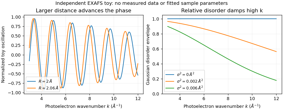
Bond distance and disorder affect EXAFS differently
. Original independent toy signals: distance changes oscillation phase, while Gaussian relative disorder damps the high-wavenumber envelope. Curves are not fits to the exam spectra or measurements. Details. Past exam of the formation of Structure in the Universe course of the University of Cambridge 2012 Paper 1 3 Solution by Codex 0 2026-10-20
Codex 0 2026-10-20The normalized cycloid hasThe initially expanding perturbation reaches maximum radius at , , then formally collapses to zero radius at , . A finite virialized object is assigned the conventional formation epoch ; random motions replace the pressureless point-collapse singularity. The cycloid alone does not describe that relaxation.
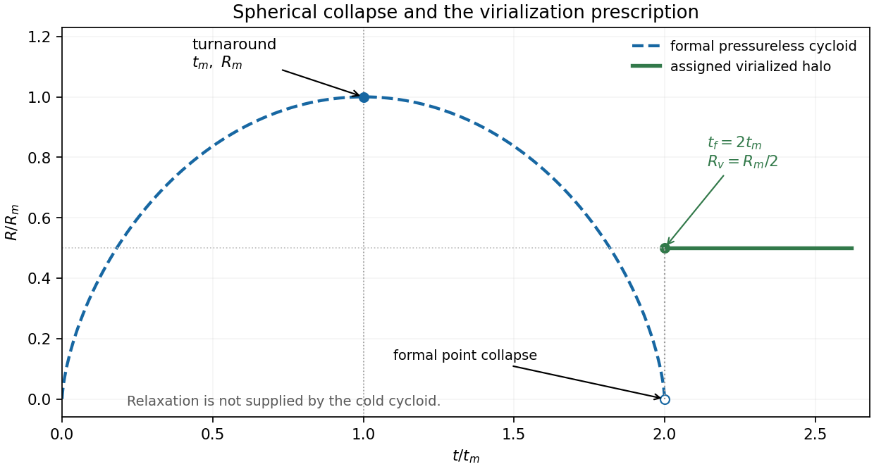
For the standard top-hat virialization estimate, write and retain the same gravitational structure factor at turnaround and final equilibrium. The coherent kinetic energy vanishes at turnaround, whereas the virial theorem gives in the final isolated equilibrium. conservation of energy givesThe final density is eight times the turnaround density. Meanwhile , so . The Einstein-de Sitter virial overdensity follows by combining these factors with the supplied turnaround contrast:The value 200 is a convenient rounded overdensity convention, not exactly the Einstein-de Sitter result.
The virial radius of a dark-matter halo follows from :The hydrostatic temperature of an inverse-square halo follows from hydrostatic equilibrium and the ideal gas law:Since and , cancellation of gives . ThereforeHere is a dimensionful mean particle mass, as specified in the paper; a dimensionless mean molecular weight would need multiplication by a particle-mass unit. The isothermal interior is a further halo idealization, not an exact continuation of the uniform top-hat profile used in the virial-overdensity estimate. Changing its gravitational structure factor in a literal energy comparison would change the turnaround-radius relation.
The formation redshift from halo mean density uses the cluster data, which imply . Thus, using the requested rounded convention,Using instead gives . In the Einstein-de Sitter time scaling the rounded-convention result is . Directly from the mass and radius,For the estimate, take mean particle mass , appropriate approximately to a hydrogen-helium mixture with complete ionization. This gives , or . The composition choice is additional input, not a value supplied by the examination; the boxed expression retains the result for any .
Pinned article: Introduction to the OurBigBook Project
Welcome to the OurBigBook Project! Our goal is to create the perfect publishing platform for STEM subjects, and get university-level students to write the best free STEM tutorials ever.
Everyone is welcome to create an account and play with the site: ourbigbook.com/go/register. We belive that students themselves can write amazing tutorials, but teachers are welcome too. You can write about anything you want, it doesn't have to be STEM or even educational. Silly test content is very welcome and you won't be penalized in any way. Just keep it legal!
Intro to OurBigBook
. Source. We have two killer features:
- topics: topics group articles by different users with the same title, e.g. here is the topic for the "Fundamental Theorem of Calculus" ourbigbook.com/go/topic/fundamental-theorem-of-calculusArticles of different users are sorted by upvote within each article page. This feature is a bit like:
- a Wikipedia where each user can have their own version of each article
- a Q&A website like Stack Overflow, where multiple people can give their views on a given topic, and the best ones are sorted by upvote. Except you don't need to wait for someone to ask first, and any topic goes, no matter how narrow or broad
This feature makes it possible for readers to find better explanations of any topic created by other writers. And it allows writers to create an explanation in a place that readers might actually find it.
Figure 1. Screenshot of the "Derivative" topic page. View it live at: ourbigbook.com/go/topic/derivativeVideo 2. OurBigBook Web topics demo. Source. - local editing: you can store all your personal knowledge base content locally in a plaintext markup format that can be edited locally and published either:This way you can be sure that even if OurBigBook.com were to go down one day (which we have no plans to do as it is quite cheap to host!), your content will still be perfectly readable as a static site.
- to OurBigBook.com to get awesome multi-user features like topics and likes
- as HTML files to a static website, which you can host yourself for free on many external providers like GitHub Pages, and remain in full control

Figure 2. You can publish local OurBigBook lightweight markup files to either OurBigBook.com or as a static website.
Figure 3. Visual Studio Code extension installation.
Figure 5. . You can also edit articles on the Web editor without installing anything locally. Video 3. Edit locally and publish demo. Source. This shows editing OurBigBook Markup and publishing it using the Visual Studio Code extension. 
- Infinitely deep tables of contents:




All our software is open source and hosted at: github.com/ourbigbook/ourbigbook
Further documentation can be found at: docs.ourbigbook.com
Feel free to reach our to us for any help or suggestions: docs.ourbigbook.com/#contact