The incident plane wave is periodic in $\theta$, so expand it as a Fourier series ${\sum }_m{R}_m(r)e^{im\theta }$. Substitution into the Helmholtz equation, with $\rho =kr$, gives the radial Bessel differential equationRegularity at the origin selects the Bessel function of the first kind, rather than the singular second solution. ThusThe coefficients $a_m$ are independent of $r$; their values follow from matching near the origin in the next part. The completed identity is the Jacobi-Anger expansion.

The incident plane wave carries probability current $j_{\mathrm{in}}=\hslash k/m$. For the separated outgoing wave from the previous part,The rate through a distant arc is $r{j}_r^{\mathrm{sc}}d\theta$. Dividing by incident flux defines the differential two-dimensional scattering cross-section,Because $f$ is dimensionless, $\lambda$ has units of length, as appropriate for scattering in a plane.

Outside a short-range scattering region, the stationary Schrödinger equation reduces to the two-dimensional Helmholtz equation. Separation in polar coordinates gives outgoing radial Hankel functions, whose large-$r$ dependence is $r^{-1/2}{e}^{ikr}$. The same power follows from conserved probability current: a circle has length proportional to $r$, so the squared outgoing amplitude must decrease as $1/r$.

For an incident plane wave in the $x$ direction, adopt the dimensionless amplitude conventionThe phase $e^{i\pi /4}$ and factor $k^{-1/2}$ specify the definition of $f$; they can be absorbed into a differently normalized scattering amplitude. Here they are kept exactly so that the later two-dimensional scattering cross-section follows consistently.

For fixed $g>0$, write $A=\hslash T/(2m)$. The bound contribution to the quantum propagator of an attractive delta potential remains $\kappa e^{i\hslash {\kappa }^{2}T/(2m)}$. For its continuum, the stationary phase is at $k=0$, where $k^2/(k^2+{\kappa }^2)=k^2/{\kappa }^2+O(k^4)$. The Gaussian oscillatory integral and its derivative giveConsequentlyThe continuum decays as $T^{-3/2}$, but the full kernel has a persistent oscillating bound state contribution and no ordinary complex limit. This expansion requires $\hslash {\kappa }^{2}T/(2m)\gg 1$; it is not uniform in the zero-coupling limit, where the bound state disappears and the free kernel instead decays as $T^{-1/2}$.

At the origin, the normalized bound state in a delta potential contributes $|{\phi }_0(0){|}^2=\kappa$, and the odd scattering eigenfunctions contribute zero. The even continuum functions from the preceding part haveTheir energy is $E_k={\hslash }^2{k}^2/(2m)$. Inserting these weights into the spectral resolution of a quantum propagator, and using evenness to extend the integral to the whole real axis, yields for $T>0$This is the quantum propagator of an attractive delta potential. The printed continuum exponent has an extra factor of $\hslash$: its time phase must be $-i{E}_{k}T/\hslash =-i\hslash k^{2}T/(2m)$. This correction also makes the exponent dimensionless. Oscillatory integrals are understood with an infinitesimal positive convergence factor before taking its limit.

Choose the even-channel scattering phase shift convention ${\phi }_{k,e}(x)={\pi }^{-1/2}\cos (k|x|+{\delta }_e)$ for $k>0$. The delta potential derivative jump givesso, choosing the branch that tends to zero as $k\to \infty$,An odd scattering eigenfunction is ${\phi }_{k,o}(x)={\pi }^{-1/2}\sin kx$: it vanishes at the interaction and its derivative is continuous, so it acquires no scattering phase shift. These parity channels, with the bound state, give the continuum part of the spectral resolution of a quantum propagator.

Away from the delta potential, the decaying bound state obeys $E_0=-{\hslash }^2{\kappa }^2/(2m)$. Integrating the Schrödinger equation across the attractive interaction givesFor an even exponential, the left side is $-2\kappa \phi (0)$. ThereforeThe normalized bound state in a delta potential is ${\phi }_0(x)=\sqrt{\kappa }{e}^{-\kappa |x|}$, since $2\kappa {\int }_0^{\infty }{e}^{-2\kappa x}dx=1$. The single positive solution for $\kappa$ gives one bound state; an odd decaying wave cannot be both continuous and nonzero with this interaction.

For a time-independent Hamiltonian operator, the time-evolution operator is $U(T)=e^{-iHT/\hslash }$, with $T=t-t^{\prime }$. Insert its resolution of identity in normalized energy eigenstates:Since $⟨x|\alpha ⟩={\phi }_{\alpha }(x)$, the retarded quantum propagator in the question isThe Heaviside step function imposes the chosen retarded convention. If the Hamiltonian operator has a continuous spectrum, the spectral sum includes its continuum integral; it must not be restricted to bound states. The spectral resolution of a quantum propagator also shows that $K$ tends to $\delta (x-x^{\prime })$ as $T\downarrow 0$. With the step factor it obeys $(i\hslash {\partial }_t-H)K=i\hslash \delta (T)\delta (x-x^{\prime })$; the corresponding Green function with a unit delta source is $K/(i\hslash )$.

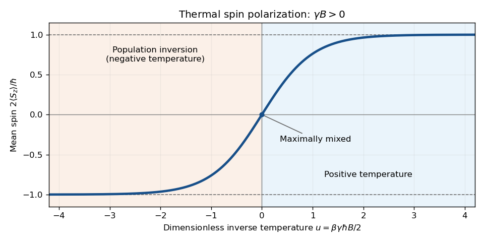
For $\mathbf{B}=B{\mathbf{e}}_z$, the quantum Gibbs state is diagonal in the $S_z$ basis. Its two probabilities are proportional to $e^{\pm \beta \gamma \hslash B/2}$. ThusAt small inverse temperature, $⟨S_z⟩\simeq \beta \gamma {\hslash }^{2}B/4$. As a function of $u=\beta \gamma \hslash B/2$, the normalized spin component is the smooth odd curve $\tanh u$: it crosses zero at $u=0$ and saturates at $\pm 1$. As a function of $\beta$ its direction is reversed if $\gamma B<0$. For $\gamma B>0$, positive temperature favors $S_z=+\hslash /2$, while negative temperature gives the inverted population.

Specify the magnetic coupling before fixing its sign: let the magnetic moment be $\mathbf{\mu }=\gamma \mathbf{S}$, where $\gamma$ is a signed gyromagnetic ratio. The Zeeman effect gives $H_Z=-\gamma \mathbf{B}\cdot \mathbf{S}$. For spin one-half, $\mathbf{S}=\hslash \mathbf{\sigma }/2$, so with $B=|\mathbf{B}|$ and $u=\beta \gamma \hslash B/2$,This is the quantum Gibbs state. Its eigenvalues are $(1\pm \tanh u)/2$, so its purity is $(1+{\tanh }^{2}u)/2$. For nonzero level splitting it approaches a pure state as $|u|\to \infty$: positive inverse temperature selects the lower energy, while negative inverse temperature selects the upper one. It is a maximally mixed state at $u=0$, including infinite temperature or zero magnetic splitting. At zero field the Gibbs state remains $I/2$; lowering temperature alone does not select a unique pure state from that degeneracy.

Negative temperature is meaningful for an internally equilibrated spin sector with a bounded energy spectrum and population inversion. It must be sufficiently isolated from unbounded motional degrees of freedom: the oscillator's unbounded spectrum, for instance, makes its partition sum diverge at negative inverse temperature. The two-level spin partition sum itself stays finite for either sign.

The quantum state is continuous through a sudden finite-force quantum quench, so it is still $|0⟩$ at $t=0^{+}$. DefineThe new Hamiltonian operator is $H=\hslash \omega (b^{†}b+1/2)-\hslash \omega {\lambda }^2$. The old Fock vacuum obeys $b|0⟩=-\lambda |0⟩$, so the coherent state after shifting an oscillator equilibrium rotates with amplitude $-\lambda e^{-i\theta }$ relative to the new equilibrium. In the original oscillator basis, the full state isOne way to obtain the phase is to writeand apply the displacement operator composition rule. The coherent-state oscillator expectation values giveThe position uncertainty stays $\sqrt{\hslash /(2M\omega )}$. These mean values obey the forced classical equation, while the nonzero variance retains the quantum width.

A normalized oscillator coherent state is an eigenstate of the annihilation operator, $a|\alpha ⟩=\alpha |\alpha ⟩$. Expanding it in Fock states givesSince $x=\sqrt{\hslash /(2M\omega )}(a+a^{†})$, $⟨a^2⟩={\alpha }^2$, and $⟨a{a}^{†}⟩=|\alpha {|}^2+1$, the variance is $⟨x^2⟩-⟨x{⟩}^2=\hslash /(2M\omega )$. Henceindependently of the complex amplitude $\alpha$.

For $A=\alpha a^{†}$ and $B=-{\alpha }^{\ast }a$, the commutator is the scalar $[A,B]=|\alpha {|}^{2}I$. The Baker--Campbell--Hausdorff formula therefore terminates and gives the displacement operatorBecause $a|0⟩=0$, applying it to the Fock vacuum yields exactly the Fock state expansion above:For a general complex $\alpha$, its complex conjugate is required in the annihilation term. The expression with $-\alpha a$ printed in the paper is valid when $\alpha$ is real.

Complete the square in the potential energy. With $x_F=F/(M{\omega }^2)$,The quantum harmonic oscillator is translated without changing its level spacing. If ${\phi }_n(x)$ is its normalized unforced energy eigenstate, thenEquivalently, $|n;F⟩=e^{-i{x}_{F}p/\hslash }|n⟩$. The ground state position is centered at $x_F$, and its position uncertainty remains $\sqrt{\hslash /(2M\omega )}$.

For distinct positive integers $p,q$, use normalized box modes ${\phi }_1=\sqrt{2/L}\sin (p\pi x/L)$ and ${\phi }_2=\sqrt{2/L}\sin (q\pi x/L)$. Their contact interaction overlaps obeyUnlike traveling ring modes, these standing modes also allow pair conversion. For the first two box modes, or any distinct pair without a third-harmonic resonance, the contact interaction between two box modes isThe last two terms change an individual mode occupation number by two while conserving total particle number. Thus the Hamiltonian operator is not diagonal in the Fock state basis, and minimizing diagonal entries alone does not find its ground state. For example, at $N=2$ with no dispersion, $\left(|2,0⟩-|0,2⟩\right)/\sqrt{2}$ has the lowest energy $g/(2L)$, below either unmixed endpoint's $3g/(2L)$.

The wording permits modes beyond the first two. For completeness, the identity ${\sin }^{3}u=(3\sin u-\sin 3u)/4$ givesWhen $q=3p$, add $-g(a_1^{†2}{a}_1{a}_2+a_1^{†}{a}_2^{†}{a}_1^2)/(2L)$; when $p=3q$, add $-g(a_1^{†}{a}_2^{†}{a}_2^2+a_2^{†2}{a}_1{a}_2)/(2L)$. These extra terms change an individual occupation number by one and require diagonalizing the corresponding fixed-$N$ matrix as well.

Add the one-particle energy term $H_0={ϵ}_1{n}_1+{ϵ}_2{n}_2$. It is diagonal in the same Fock state basis as the contact interaction between two ring modes. For $N=2$, the ordered basis $(|2,0⟩,|1,1⟩,|0,2⟩)$ givesFor $g>0$, the middle eigenvalue exceeds the mean of the two endpoint eigenvalues by $g/L$, so it cannot be the smallest. The ground state is therefore $|2,0⟩$ if ${ϵ}_1<{ϵ}_2$, and $|0,2⟩$ if ${ϵ}_2<{ϵ}_1$, withIf ${ϵ}_1={ϵ}_2$, every normalized linear combination of the two endpoint Fock states is a ground state. The same endpoint argument works for general fixed $N$, since the interaction contribution is a concave quadratic function of the mode occupation number.

At fixed particle number $N$, write $n_1=n$ and $n_2=N-n$. The contact interaction between two ring modes has energy eigenvaluesFor $g>0$, the nonnegative product $n(N-n)$ is minimized at the endpoints. ConsequentlyFor $N\ge 1$ this is a two-dimensional degenerate ground state subspace. $N=0$ instead has the unique Fock vacuum. In this projected model, putting all particles into one traveling mode avoids the extra exchange contribution paid when both distinct modes are occupied.

For the alternative coefficients, put $\alpha =\beta =A<0$ and $\gamma =0$. Then $E(n)=A[N(N-1)-2n(N-n)]$ is again minimized at $n=0,N$, with $E_{\min }=AN(N-1)$. Evenness of $N$ is unnecessary for this result; the balanced Fock state maximizes this attractive-interaction energy instead of minimizing it.

Normalize the ring modes as ${\phi }_j(x)=L^{-1/2}{e}^{i{k}_{j}x}$, with distinct $k_j=2\pi {\ell }_j/L$ and integers ${\ell }_j$. Inserting $\hat{\psi }(x)={\phi }_1(x)a_1+{\phi }_2(x)a_2$ into the contact interaction givesOrthogonality makes $I_{ijkl}=1/L$ when $k_i+k_j=k_k+k_l$, and zero otherwise: this is momentum conservation in the projected Hamiltonian operator. There is one all-mode-1 term, one all-mode-2 term, and four mixed terms with one particle in each mode. A pair conversion between distinct ring modes would require $2k_1=2k_2$ and therefore vanishes.

Using $a_j^{†2}{a}_j^2=n_j(n_j-1)$ and $a_1^{†}{a}_2^{†}{a}_1{a}_2=n_1{n}_2$ yields the contact interaction between two ring modes,The factor four comes from two independent choices of ordering for the creation operators and annihilation operators. This is the two-mode projected model; a full ring contact interaction can also scatter particles into other modes while conserving total momentum.

In second quantization, expand the annihilating quantized field in a complete orthonormal basis of one-particle states, $\hat{\psi }(x)={\sum }_{\alpha }{\phi }_{\alpha }(x)a_{\alpha }$. At equal times, the canonical commutation relation for bosons and the canonical anticommutation relations for fermions are, respectively,andHere $\delta$ is a Dirac delta distribution. Multiplying by the basis wave functions and integrating gives $[a_{\alpha },a_{\beta }^{†}]={\delta }_{\alpha \beta }$ for bosons, or $\{a_{\alpha },a_{\beta }^{†}\}={\delta }_{\alpha \beta }$ for fermions; the two-annihilator and two-creator brackets vanish in the corresponding convention.

The mode number operator and total particle number operator areThe bosonic occupation numbers are $0,1,2,\dots$. For fermions, $a_{\alpha }^2=0$ and the canonical anticommutation relations imply $n_{\alpha }^2=n_{\alpha }$, so the fermionic occupation numbers are only $0$ and $1$, as required by the Pauli exclusion principle.

Keeping only two modes later is a projection: the projected field bracket is ${\sum }_{j=1}^2{\phi }_j(x){\phi }_j^{\ast }(x^{\prime })$, rather than the full Dirac delta distribution.

Above the threshold, $c^2{k}_j^2>1/(4{\tau }^2)$, the square root in part (d) is real. Both fields oscillate, but the first has envelope $\boxed{e^{-t/(2\tau )}}$ and the second $\boxed{e^{+t/(2\tau )}}$. Thus the first is damped and the second amplified.

Below the threshold, set ${\sigma }_j=\sqrt{1/(4{\tau }^2)-c^2{k}_j^2}$. The temporal factors areThey are nonoscillatory. For nonzero $k_j$, $0<{\sigma }_j<1/(2\tau )$, so both first-field branches decay and both second-field branches grow. At $k_j=0$, one branch is constant; the other is $e^{-t/\tau }$ for ${\varphi }_1$ or $e^{t/\tau }$ for ${\varphi }_2$.

At equality, the repeated temporal root gives $\boxed{(A+Bt)e^{-t/(2\tau )}}$ for the first field and $\boxed{(C+Dt)e^{t/(2\tau )}}$ for the second. The full two-field system is generically unstable on both sides because of the amplified sector. This is compatible with its autonomous Lagrangian: the total conserved energy is an indefinite quadratic form, rather than a positive energy forcing every component to remain bounded.

The velocity coupling changes the momenta and the undifferentiated field terms. Variation with respect to ${\varphi }_2$ gives the equation for ${\varphi }_1$:so the two Euler-Lagrange field equations areThey describe damped and antidamped fields from an antisymmetric velocity coupling. With the convention ${\varphi }_j=A_j{e}^{i(k_{j}x-{\omega }_{j}t)}$, their characteristic equations areThus the dispersion relations and modes areFor each spatial Fourier mode, the general solution is the linear combination of its two temporal branches; spatial superposition gives the general field. Take real parts or suitable complex conjugate pairs to obtain the required real fields. At the repeated-root threshold, the independent second temporal solution contains an extra factor $t$, as detailed next.