With constant $\nu$, the bulk action is invariant under time translations, translations in the two spatial coordinates, and rotations or reflections within the substrate plane. The Laplacian has no preferred direction, giving the planar $O(2)$ symmetry. It also has scalar-field shift symmetry $h\mapsto h+a$, expressing the arbitrary origin of height, and the discrete symmetry $h\mapsto -h$ because its residual is squared.

There is an additional exact tilt symmetry $h\mapsto h+\mathbf{b}\cdot \mathbf{x}$: the added slope is time independent and has zero Laplacian. More generally, adding any function $f$ satisfying $f_t=\nu {\nabla }^{2}f$ leaves the residual unchanged. Such bulk transformations need not preserve prescribed boundary conditions or a restricted physical interpretation of the height.

In two spatial dimensions the action also has the anisotropic scale invarianceThe spacetime measure scales as $b^4$ and the squared residual as $b^{-4}$. The time and length scales are therefore related diffusively, rather than by a Lorentz transformation.

Ordinary time reversal needs a boundary qualification. The identityshows that the density is time-reversal invariant up to a total divergence. Thus the bulk stationary equation $h_{tt}-{\nu }^2{\nabla }^{4}h=0$ is invariant under $t\mapsto -t$, although the printed density is not pointwise unchanged. The time reversal of the squared diffusion-residual action exchanges the growing and decaying branches; the selected first-order diffusion equation alone is not time-reversal invariant at fixed positive $\nu$.

Put $R=h_t-\nu {\nabla }^{2}h$, where the diffusion coefficient $\nu$ is constant. ThenOne temporal and two spatial integrations by parts givewith compactly supported variations. HenceHere ${\nabla }^4=({\nabla }^2{)}^2$ is the biharmonic operator. The cross terms cancel because $\nu$ is constant and spatial and temporal derivatives commute. Equivalently, $P^0=2R$ and $Q^{ij}=-2\nu R{\delta }^{ij}$ in part (b), producing $-2{\partial }_{t}R-2\nu {\nabla }^{2}R=0$.

This squared diffusion-residual action does not have only the first-order diffusion equation as its stationary equation. The zero-residual paths $h_t=\nu {\nabla }^{2}h$ have $S=0$ and are certainly solutions, but the variational equation is the higher-order one above. For a spatial Fourier mode with nonzero wavevector $\mathbf{k}$, it givesBoundary data or an additional physical selection principle are needed to retain only the decaying diffusion branch. The spatially uniform mode instead has $h_0(t)=A_0+B_{0}t$ in the stationary equation.

Let $P^{\mu }=\partial \mathcal{L}/\partial ({\partial }_{\mu }h)$ and $Q^{\mu \nu }=\partial \mathcal{L}/\partial ({\partial }_{\mu }{\partial }_{\nu }h)$. Define the second coefficient with ordered repeated indices and $Q^{\mu \nu }=Q^{\nu \mu }$, so thatThis convention avoids double-counting a mixed derivative such as $h_{,12}=h_{,21}$. The first derivative term needs one integration by parts. The second derivative term needs two:Combining the terms givesFor compactly supported variations, or fixed $\delta h$ and its first derivatives at the boundary, the last integral vanishes. The fundamental lemma of the calculus of variations then yields the Euler-Lagrange field equation with second derivatives:The plus sign of the final term comes from the two integrations by parts. In general this gives fourth-order equations, although the order in a particular coordinate depends on which second derivatives occur in the density.

If $L^{\prime }=L+dF(q,t)/dt$, the action changes by an endpoint term:In the principle of stationary action with fixed endpoints, $\delta q(t_i)=\delta q(t_f)=0$ and the endpoint times are fixed. Therefore $\delta (S^{\prime }-S)=0$, and the two actions give the same bulk Euler-Lagrange equations.

For a Lagrangian density, adding ${\partial }_{\mu }{K}^{\mu }$ changes the action by ${\int }_{\partial \Omega }{K}^{\mu }{n}_{\mu }d\Sigma$, by the divergence theorem. Its variation vanishes for compactly supported field variations, or when the appropriate boundary data are held fixed. These total divergences in a variational principle can therefore be discarded when deriving bulk equations under those conditions.

The qualification about boundaries matters: if $K^{\mu }$ depends on field derivatives, their variations on the boundary must also be controlled. A total derivative can change the canonical momenta or the chosen representative of a Noether current, even while leaving the bulk dynamics unchanged.

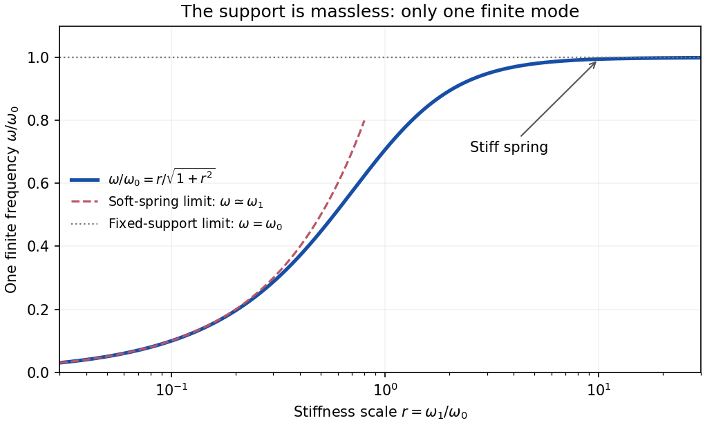
Subtracting the two linearized equations eliminates their acceleration terms:For $g,k>0$, the assumed nontrivial simple harmonic motion therefore hasThe support displacement and pendulum angle oscillate in phase. Inserting this relation into either Euler-Lagrange equation yieldsso the one positive finite angular frequency isThe negative frequency describes the same real oscillation after a phase change. For a general phase, replace the sine in both coordinates by $A\cos (\omega t)+B\sin (\omega t)$.

There is no missing second finite branch. The quadratic Lagrangian iswhose kinetic matrix is $\left(\begin{array}{cc}1& 1\\ 1& 1\end{array}\right)$ and has rank one. Its characteristic determinant is ${\omega }_0^2{\omega }_1^2-({\omega }_0^2+{\omega }_1^2){\omega }^2$, not a quadratic polynomial in ${\omega }^2$. This singular kinetic matrix in small oscillations results from taking the support mass to be exactly zero. Adding a small support mass restores a second mode that runs to infinite frequency as that mass vanishes.

For a stiff spring,The hinge becomes fixed, recovering the simple pendulum frequency, as expected for the pendulum with a massless spring-mounted support. At finite $k$, horizontal support motion makes the frequency smaller.

For the horizontal generalized coordinate $\eta$,The corresponding Euler-Lagrange equation isFor $\theta$, the terms proportional to $\dot{\eta }\dot{\theta }\sin \theta$ cancel between $d(\partial L/\partial \dot{\theta })/dt$ and $\partial L/\partial \theta$. Hence the other exact equation isKeeping only terms linear in small coordinates and their derivatives givesThe equilibrium is $\theta =\eta =0$. These characteristic frequencies label gravitational and spring restoring scales; they are not two independent normal mode frequencies of this massless-support system.

Use the downward $y$ direction of the PDF diagram. The bob's Cartesian coordinates areThusThe hinge and rod are massless, so only the bob contributes kinetic energy:Because gravity points along positive $y$, its gravitational potential energy is $-mgy=-mg\ell \cos \theta$. The zero-rest-length spring has elastic potential energy $k{s}^2/2$. Put $s=\ell \eta$ and divide $T-V$ by the positive constant $m{\ell }^2$. The equivalent Lagrangian isMultiplying the action by a nonzero constant leaves its stationary paths unchanged. This derivation is a direct use of kinetic energy from Cartesian position vectors; no independent kinetic term should be assigned to the massless support.

Let $\mathbf{b}=\mathbf{B}/B$ for a nonzero constant magnetic field. Since $\gamma$ is constant, the relativistic Lorentz force reduces toThe projection along $\mathbf{b}$ is constant. In the perpendicular plane define the signed cyclotron frequency $\Omega =eB/(m{\gamma }_0)$; thenThe explicit rotating velocity isThis is the relativistic cyclotron orbit frequency in laboratory time, reduced from the nonrelativistic frequency by $1/{\gamma }_0$. With nonzero parallel velocity, the trajectory is a helix. If ${\mathbf{v}}_{\perp 0}=0$, that perpendicular vector stays zero and has no nontrivial fundamental period; the displayed $T$ is the period of a nonzero transverse orbit.

With no electric field, the power relation from part (a) givesConsequentlyThe magnetic part of the relativistic Lorentz force changes the direction of mechanical momentum, but performs no work. This conclusion does not require the magnetic field to be spatially uniform: it follows from the local orthogonality of $\mathbf{v}$ and $\mathbf{v}\times \mathbf{B}$.

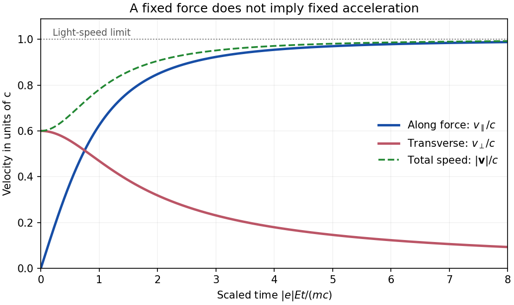
If $e\mathbf{E}\ne 0$, then $\mathbf{p}(t)=e\mathbf{E}t+O(1)$, and the relativistic energy-momentum relation givesThe particle approaches the speed of light in the direction of the electric force, independently of its initial velocity. For positive $e$ the limiting direction is along $\mathbf{E}$; for negative $e$ it is opposite. A massive particle never reaches that limiting speed in finite time. If the force is zero, the velocity remains ${\mathbf{v}}_0$ instead.

For a uniform constant electric field and zero magnetic field, the mechanical momentum changes linearly even though the velocity does not:Invert $\mathbf{p}=m\gamma \mathbf{v}$ using $\gamma =\sqrt{1+p^2/(m^2{c}^2)}$. The result for arbitrary initial direction isEquivalently, $\mathbf{v}=c\mathbf{p}/\sqrt{m^2{c}^2+p^2}$. This gives $\mathbf{v}(0)={\mathbf{v}}_0$ and guarantees $|\mathbf{v}|<c$ at every finite momentum. The transverse momentum stays constant, but its velocity component generally decreases because the Lorentz factor increases. Thus an initial transverse velocity must not be treated as constant during the electric acceleration; this is the relativistic motion in a constant electric field with transverse momentum effect.

Choose Minkowski metric $(+,-,-,-)$, so $A_{\mu }=(\varphi /c,-\mathbf{A})$ and $d\tau =dt\sqrt{1-v^2/c^2}$. In laboratory time the relativistic charged-particle action has LagrangianHere $e$ denotes the signed particle charge in the action. The canonical momentum and the position derivative areThe Euler-Lagrange equation therefore givesThe last term is $(\mathbf{v}\times \mathbf{B}{)}_i$, and the first two terms form the electric field. Thus the relativistic Lorentz force equation isIts power relation and acceleration form areThe power relation follows by taking the scalar product with $\mathbf{v}$ and using the relativistic energy-momentum relation. It also shows why the magnetic field alone cannot change the particle's energy.

Substitute $\omega ={\alpha }_3/\epsilon +\cdots$ into the cubic denominator. Its leading terms areThe nonzero large root obeys $1+i{\alpha }_3=0$, soThe sum of the three roots is exactly $i/\epsilon$. Combining this with the two slow-root expansions gives the refinement ${\omega }_3=i/\epsilon +i\epsilon +O({\epsilon }^3)$.

For physical radiative sign $\epsilon >0$, the fast pole lies high in the upper half-plane. Its homogeneous mode is $e^{-i{\omega }_{3}t}\simeq e^{t/\epsilon }$, a runaway. It prevents a bounded retarded response with the real-axis Fourier prescription even though the two slow poles are damped. If $\epsilon <0$, the fast pole decays but the slow pair grow. No nonzero real sign puts every pole in the lower half-plane.

There are two distinct boundary choices. A strictly causal initial-value Green function exists and includes the growing mode for $\epsilon >0$; it must be represented by a Laplace/Bromwich contour above that pole rather than the stated ordinary Fourier integral. Alternatively the real-axis inverse gives a bounded stationary no-runaway response and preacceleration: for $\tau <0$, upper closure encloses the fast pole and yields a nonzero response before the force. Its leading contribution isThis follows from the upper-pole residue $\mathrm{Res}G\simeq -i\epsilon$ and the factor $i$ from upper contour closure. Eliminating runaway growth by a future boundary condition therefore sacrifices strict retardation on the short scale $\epsilon$.

The singular root also shows why a perturbative expansion around only $\omega =\pm 1$ misses the problem. For a low-frequency effective description, order reduction of a radiation-reaction oscillator uses $\stackrel{...}{x}\simeq \dot{f}-\dot{x}$ in the small correction and gives $\ddot{x}+\epsilon \dot{x}+x=f+\epsilon \dot{f}$. For positive $\epsilon$ this approximate second-order equation has a causal damped response and discards the fast mode outside its intended regime; it does not make the original third-order equation simultaneously bounded and retarded.

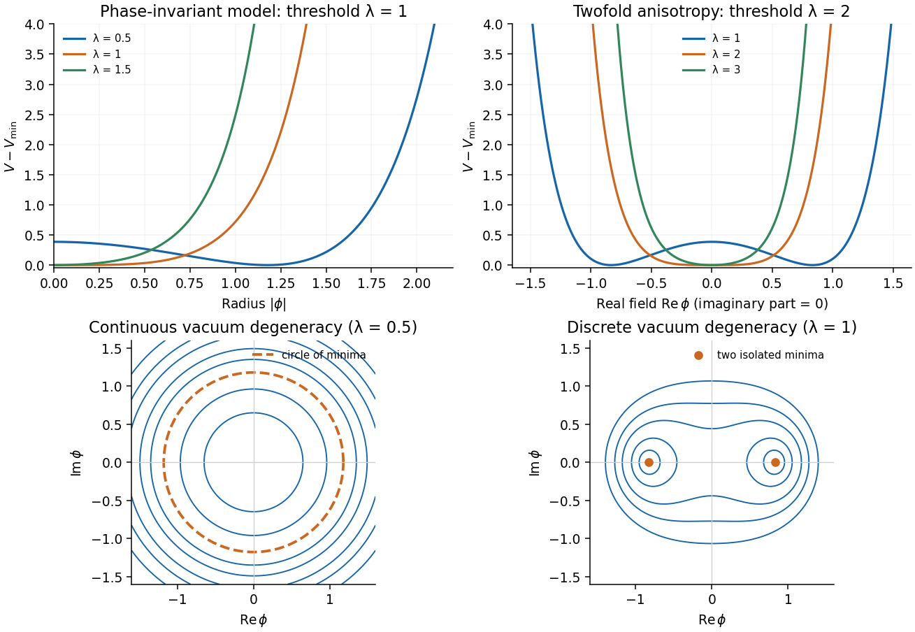
Write $\varphi =x+iy$. The added term is $-(x^2-y^2)$, so the full potential simplifies toThe phase-rotation subgroup is reduced from U(1) to the two-element symmetry $\varphi \mapsto -\varphi$. More fully, the kinetic term and potential are invariant under independent reflections $x\mapsto -x$ and $y\mapsto -y$, a ${\mathbb{Z}}_2\times {\mathbb{Z}}_2$ internal symmetry generated by $\varphi \mapsto -\varphi$ and complex conjugation. There is no continuous internal rotation symmetry for the explicit twofold anisotropy of a complex scalar field.

For fixed $x$, positive $\lambda$ makes the exponential grow with $y^2$, so every global minimum has $y=0$. On the real axis,ThusFor $0<\lambda <2$, the nonzero stationary points are the two global minima; the origin is unstable along the real direction. For $\lambda \ge 2$ the origin is the unique minimum, with zero real-direction quadratic curvature at the critical value $2$. Selecting $+v$ breaks the sign reversal that exchanges the two vacua, while complex conjugation remains unbroken.

Set $\varphi =v+\chi$, $\chi =u+iw$. Since $e^{\lambda v^2}=2/\lambda$, expansion givesEquivalently, in canonical fields $h=\sqrt{2}u$, $\pi =\sqrt{2}w$,Both masses are positive throughout the broken phase $0<\lambda <2$. A broken discrete symmetry does not demand a massless Goldstone boson. At $\lambda =2$ the radial mass tends to zero at a phase boundary, so a claim of strictly positive mass there would be incorrect. For completeness, expanding around the symmetric origin gives squared masses $\lambda -2$ and $\lambda$ for the canonical real and imaginary fields.

Write $\varphi =(v+h/\sqrt{2})e^{i\vartheta }$. The covariant kinetic term containsA local U(1) gauge symmetry can remove $\vartheta$ in unitary gauge. The angular fluctuation no longer appears as an independent physical massless Goldstone boson; its degree of freedom supplies the longitudinal polarization of the massive vector field. At quadratic order,The factor of two follows from the convention that $v$ is the complex field's vacuum value. This Higgs mechanism changes a two-polarization massless electromagnetic field into a three-polarization massive Proca field; the remaining radial scalar keeps $m_h^2=2\lambda v^2$. Static fields in the homogeneous broken phase are screened on a scale of order $m_A^{-1}$ in these units. The gauge symmetry is a redundancy of the description; the physical statement is the changed spectrum and disappearance of an independent massless angular mode.

Let $v=\sqrt{-\ln \lambda /\lambda }>0$ and write $\varphi =v+\chi$. ThenSince $V^{\prime }(v^2)=0$ and $V^{\prime \prime }(v^2)=\lambda$, the quadratic potential isThereforeThe constant can be dropped from the fluctuation equations. For canonical real fields, use $\chi =(h+i\pi )/\sqrt{2}$:These are the radial and angular masses of a phase-invariant scalar potential. The radial Higgs mode changes the field magnitude and costs energy to second order. The angular Goldstone boson changes the phase along the vacuum circle without a quadratic restoring force. Its linear dispersion is ${\omega }^2=|\mathbf{k}{|}^2$, whereas the radial mode has ${\omega }^2=|\mathbf{k}{|}^2+m_h^2$. The zero angular mass follows the continuous broken global symmetry, not from an accidental cancellation in a particular coordinate choice.

Use metric signature $(+,-,-,-)$ and the model's rescaled units $c=\hslash =1$. Its exponential implicitly uses dimensionless rescaled field and coupling combinations; the numerical coefficients of the potential are those supplied. Treat $\varphi$ and ${\varphi }^{\ast }$ as independent variables in taking canonical derivatives:The Hamiltonian density isThe kinetic and gradient terms are nonnegative, so a static homogeneous minimum is obtained by minimizing the potential. Put $s=|\varphi {|}^2\ge 0$. For $\lambda =0$, $V=1-s$ is unbounded below. For $\lambda <0$, the exponential decays while $-s$ tends to minus infinity. Thus a stable vacuum requires $\boxed{\lambda >0}$.

For positive $\lambda$,The exponential complex-scalar potential consequently hasFor $0<\lambda <1$, the minima form a circle $\varphi =v{e}^{i\theta }$, with $v^2=-\ln \lambda /\lambda$ and $V_{\min }=(1+\ln \lambda )/\lambda$. For $\lambda \ge 1$ the minimum has $V_{\min }=1$. The symmetry remains global phase rotation in either phase, but a chosen nonzero vacuum breaks it spontaneously. At $\lambda =1$ the origin is a unique minimum with vanishing quadratic curvature and a positive leading quartic term; this critical masslessness should not be confused with a Goldstone mode.

Define the positive focusing frequencyIn the paraxial approximation $w\simeq v$, traversal time is $T\simeq l/v$. The exit values areAcross the exit fringe, $p_{\theta }=0$ and $A_{\theta }\to 0$ remove the azimuthal velocity. The radial velocity remains continuous in the thin-fringe model. Outside, the transverse trajectory is therefore straight along a fixed azimuth, not a continuing helix. Taking the outgoing axial speed also as $v$, the distance to the axis isIt is independent of ${\rho }_0$, so all equal-speed paraxial rays focus to a common point. The condition $0<\omega l/v<\pi /2$ ensures the first focus lies beyond the exit. For a weak lens, $\boxed{f\simeq 4({\gamma }_{v}mv{)}^2/(q^2{B}^{2}l)}$.

The relativistic solenoid magnetic lens focuses either charge sign, while its rotation reverses with $qB$. Keeping the exact radius-dependent $w$, or the exit axial-speed change, produces radius-dependent corrections and spoils an exact common focus. Thus the requested focus is appropriately a paraxial result, with the end fields included even when their axial-speed changes are neglected.