Use the angular coordinate $\theta$ for the position on the ring. The kinetic energy is $T=m{a}^2{\dot{\theta }}^2/2$. The gravitational potential energy is constant because the ring is horizontal, and the ideal constraint force has no tangential component. Thus the Lagrangian has no dependence on $\theta$ itself: it is a cyclic coordinate.

The Euler-Lagrange equation givesEquivalently, the conserved conjugate momentum $p_{\theta }=m{a}^2\dot{\theta }$ is the vertical angular momentum, as required by rotational symmetry.

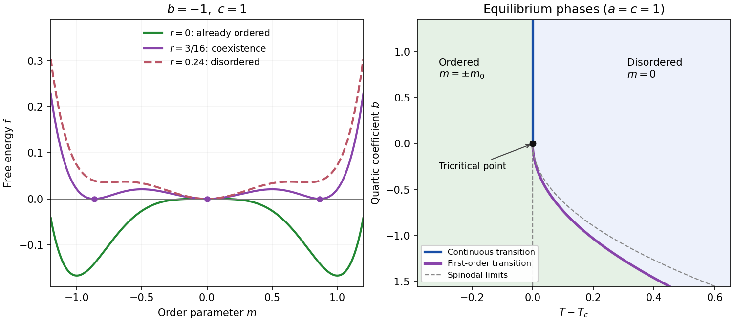
Let $\Delta T=T-T_c$, with $a,c>0$ fixed. The equilibrium phase diagram has boundariesFor either branch, larger $\Delta T$ is disordered and smaller $\Delta T$ is ordered. Both signs of the ordered magnetization are symmetry-related global minima throughout the ordered region, rather than separate regions selected by temperature and $b$.

The branches meet at the tricritical point $(\Delta T,b)=(0,0)$. Directly on $b=0$, minimizing $r{m}^2+c{m}^6/3$ givesThe transition there remains continuous, with a different mean-field critical exponent. For $b<0$, the metastability boundaries are $\Delta T=0$ for the disordered state and $\Delta T=b^2/(4ac)$ for the ordered state. The first-order phase transition curve lies strictly between them, as shown in the figure. These spinodal curves describe possible hysteretic continuation of local minima, not equilibrium phase boundaries.

At phase coexistence, the finite ordered global minimum has the same free energy as $m=0$. With $x=m^2>0$ and $f(0)=0$, stationarity and equal values giveSubtracting eliminates $r$:Substitute back to get $r_{\ast }=3b^2/(16c)$, soThe three degenerate equilibrium values at this temperature are $0$ and $\pm m_{\mathrm{jump}}$. A useful global check, avoiding confusion with a spinodal point, is the exact factorizationAll three zeros are therefore global minima. Their curvatures are positive: $f^{\prime \prime }(0)=3b^2/(8c)$ and $f^{\prime \prime }(\pm m_{\mathrm{jump}})=3b^2/(2c)$.

The ordered local minimum first appears on cooling at $r=b^2/(4c)$, where the nonzero stationary roots merge. It becomes globally stable only at $r_{\ast }$; the disordered minimum remains metastable down to $r=0$. These different temperatures distinguish phase coexistence from loss of local stability.

For $b<0$ at $T=T_c$, the quartic term lowers the free energy near $m=0$, while the positive sextic term stabilizes it at larger $|m|$. The nonzero stationary points haveThey are global minima. The stationary point $m=0$ has zero quadratic curvature but is a flat local maximum because its leading nonzero term is negative. Thus the system is already ordered at $T_c$, with a finite magnetization.

More explicitly, a continuous onset from $m=0$ could occur only where $f^{\prime \prime }(0)=2r$ vanishes, namely at $r=0$. But the global minima there are the finite values above. For sufficiently large positive $r$, only $m=0$ is stable. Therefore the equilibrium minimum must change at some positive $r$ by crossing between a zero and a finite nonzero order parameter. This is a first-order phase transition. Its actual temperature lies above $T_c$ and is calculated next; $T_c$ itself is the disordered spinodal point, not the coexistence temperature.

The stationary points of the Landau free energy obeyFor $b>0$, $r\ge 0$ makes every term of $f$ nonnegative, so $m=0$ is the unique global minimum. For $r<0$, its curvature $f^{\prime \prime }(0)=2r$ is negative. Setting $x=m^2$ gives $c{x}^2+bx+r=0$, whose unique positive root isAt a nonzero stationary point,Thus both $m=\pm \sqrt{x_{+}}$ are stable and have lower free energy than $m=0$. The equilibrium magnetization isFor fixed $b>0$ and $T\to T_c^{-}$, expand the square root:It tends continuously to zero. Hence the continuous phase transition has the order-parameter critical exponentThis is the mean-field critical exponent; fluctuation corrections beyond Landau theory are not included.

A Landau free energy is a coarse-grained thermodynamic potential expressed as a function of a proposed macroscopic order parameter. Its coefficients include microscopic and thermal effects already averaged over. At fixed external thermodynamic conditions, equilibrium selects its global minimum; other local minima can represent metastable states. It is not the internal energy of a single microscopic magnetic configuration. Here the real scalar $m$ represents a selected component of magnetization: zero describes the disordered state, while nonzero values distinguish two oppositely ordered states.

Every power is even, so the internal discrete symmetry isFor a magnetic order parameter, this represents reversal of the magnetization, as under time reversal in zero applied magnetic field. A nonzero field would generally add an odd term and break this symmetry explicitly. This scalar model has no continuous internal rotation symmetry; physical rotational symmetry of a vector magnet is not implied by treating one real component. The condition $c>0$ makes the polynomial bounded below at large $|m|$.

For the requested ordered phase on cooling, take the usual implicit assumption $a>0$, and write $r=a(T-T_c)$. If $a<0$ the temperature directions reverse; if $a=0$ this expansion has no temperature-driven transition. The source explicitly states only $c>0$.

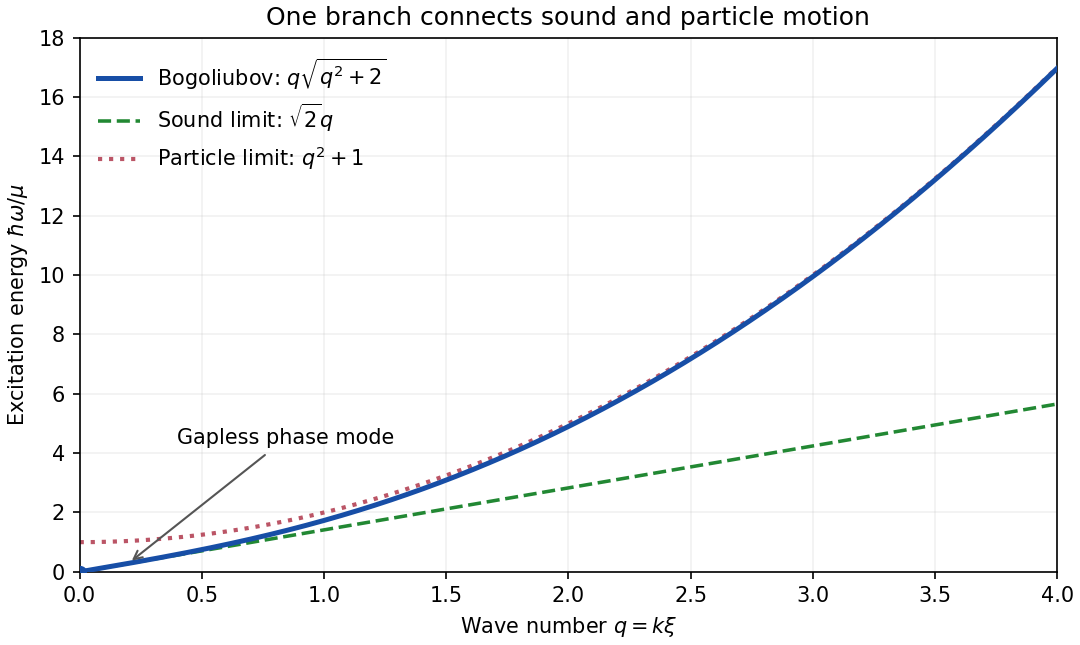
At long wavelength,This is the sound-like Goldstone mode of the broken global $U(1)$ continuous symmetry. A spatially uniform infinitesimal phase change is $\delta \psi =i{\psi }_0\delta \theta$, entirely in the ${\chi }_2$ direction, and costs no potential energy. Slow spatial variations acquire gradient energy and propagate as sound. Thus the dispersion relation realizes Goldstone's theorem through a gapless excitation; it is not a massive phase oscillation.

The amplitude and phase are canonically paired by the first-order time derivative in the quadratic condensate fluctuation Lagrangian. There is one positive-frequency branch, rather than an additional independent amplitude branch of a relativistic second-order-time theory. At high momentum,so the same branch becomes particle-like. The healing length $\xi =\hslash /\sqrt{2M\mu }$ sets the crossover scale.

For independent $\chi ,{\chi }^{\ast }$, the derivatives needed in the ${\chi }^{\ast }$ Euler-Lagrange field equation areConsequently the two conjugate field equations areWrite $\chi ={\chi }_1+i{\chi }_2$ with real components, and put $A={\hslash }^2/(2M)$. Separating real and imaginary parts givesFor each real field take the real part of a complex plane wave amplitude, ${\chi }_j=\mathrm{Re}[q_j{e}^{i(\mathbf{k}\cdot \mathbf{r}-\omega t)}]$. With ${ϵ}_k={\hslash }^2|\mathbf{k}{|}^2/(2M)$ the two equations becomeA nonzero normal mode requires their determinant to vanish, soThe positive-frequency Bogoliubov quasiparticle dispersion is thereforeThere is also the negative-frequency conjugate solution, as required for real component fields. Since $\mu >0$, ${\omega }^2\ge 0$, consistent with the stability of the chosen uniform ground state.

Choose the real representative $v={\psi }_0=\sqrt{\mu /g}$. For $\psi =v+\chi$,and the fourth power through quadratic order isIn $\mu |\psi {|}^2-g|\psi {|}^4/2$, the linear terms and the $|\chi {|}^2$ terms cancel because $g{v}^2=\mu$. The remaining potential contribution is ${\mu }^2/(2g)-\mu (\chi +{\chi }^{\ast }{)}^2/2$.

The time-derivative contribution isIts first term is a total derivative and contributes only a temporal boundary term for fixed endpoint fields. Since $v$ is uniform, the gradient contribution is simply $-{\hslash }^2|\nabla \chi {|}^2/(2M)$. Dropping that boundary term and the constant, the quadratic condensate fluctuation Lagrangian isThe omitted cubic and quartic interactions describe scattering between these small fluctuations; they do not enter the linear normal mode calculation.

Treat $\psi ,{\psi }^{\ast }$ independently in the Legendre transform in mechanics. Their canonical momenta areThe time-derivative terms cancel in ${\pi }_{\psi }\dot{\psi }+{\pi }_{{\psi }^{\ast }}{\dot{\psi }}^{\ast }-\mathcal{L}$, giving the Hamiltonian densityThe first-order time dependence makes the momenta constrained; this direct calculation still gives the canonical density. In physical terms this is the grand-canonical Hamiltonian of a Bose field, $K=H-\mu N$. The physical energy density is obtained by adding $\mu |\psi {|}^2$ back. A stationary field in this chemical-potential frame has the usual factor $e^{-i\mu t/\hslash }$ in the physical frame.

Complete the square:For uniform or periodic boundary conditions, or in the homogeneous bulk, both nonconstant terms are nonnegative and vanish simultaneously atThe ground states form a circle. A particular nonzero ${\psi }_0$ is changed by every nontrivial phase rotation, although the full family is invariant. Selecting one such mean-field theory state therefore exhibits spontaneous symmetry breaking of $U(1)$. This describes phase selection in the thermodynamic limit; an exact finite-system particle-number eigenstate need not itself have a nonzero field expectation.

Under $\psi \mapsto e^{i\alpha }\psi$ with constant real $\alpha$, the field and its complex conjugate acquire opposite phases. These cancel in $|\psi {|}^2$, $|\psi {|}^4$, $\nabla {\psi }^{\ast }\cdot \nabla \psi$, and ${\psi }^{\ast }\dot{\psi }-\psi {\dot{\psi }}^{\ast }$. The Lagrangian density therefore has the particle-number phase symmetry, a global circle group $U(1)$.

For a spacetime-dependent real $\alpha (\mathbf{r},t)$,Writing $n=|\psi {|}^2$, the change in the Lagrangian density isThis is not generally zero or a boundary term. Thus the symmetry is global, with no arbitrary local phase symmetry. A compensating gauge field and gauge-covariant derivative of a charged scalar field would be required to promote it to a local redundancy.

The constants specify isotropic, nondispersive linear response: $\kappa$ controls electric polarization, and $\chi$ controls magnetization. Their numerical relation to conventional electric susceptibility and magnetic susceptibility depends on the signs and field normalization in the action. In the rationalized units used here, the printed action gives the constitutive relationsThus its relative permittivity and magnetic permeability areHere conventional ${\chi }_m$ is defined by $\mathbf{M}={\chi }_m\mathbf{H}$, not by $\mathbf{M}={\chi }_m\mathbf{B}$. With the alternative repaired action that yields the PDF's target equation, ${\epsilon }_r$ is unchanged but ${\mu }_r=(1-\chi {)}^{-1}$ and ${\chi }_m=\chi /(1-\chi )$. In particular, a positive conventional electric susceptibility corresponds to negative $\kappa$ in the printed conventions; the problem does not specify signs for these constants.

In the rest frame $u^{\mu }=(1,0,0,0)$ and $h_{\mu \nu }=\mathrm{diag}(0,1,1,1)$. The two material contractions in the printed action become $-{\mathbf{P}}^2$ and $-2{\mathbf{M}}^2$. Consequently its material Lagrangian density isThe Euler-Lagrange field equations are algebraic, since no derivatives of the material variables occur. They giveThese also follow from the $i0$ and $ij$ components of the corrected equation in part (b). If instead the intended starting point was the PDF's displayed equation in part (b), its predictions would beThe two magnetic answers express the documented sign error, rather than different choices of frame. Here the inverse coefficients in the action require nonzero $\kappa ,\chi$; zero response is obtained as a limiting constitutive law.

Choose $A^{\mu }=(\Phi ,\mathbf{A})$, so that $F_{i0}=E_i$ and $F_{ij}={ϵ}_{ijk}{B}_k$, with ${ϵ}_{123}=1$. The definitions of the polarization-magnetization tensor imply $M^{0i}=-P_i$ and $M^{ij}={ϵ}_{ijk}{M}_k$. Separating temporal and spatial indices,The Levi-Civita symbol contraction equals $2{\delta }_{k\ell }$, givingThus $\mathbf{P}$ is the electric dipole moment per volume, or electric polarization, and $\mathbf{M}$ is the magnetic dipole moment per volume, or magnetization. The signs are those of dipole interactions in a Lagrangian; the associated fixed-dipole potential energies have the opposite signs. Consistently, the equation in part (a) has componentsso ${\rho }_b=-\nabla \cdot \mathbf{P}$ and ${\mathbf{J}}_b={\partial }_t\mathbf{P}+\nabla \times \mathbf{M}$ are the bound charge and bound current.

There is a sign inconsistency in the original PDF: varying its action gives a plus sign for the spatially projected magnetic term, whereas its displayed target equation has a minus sign. The following Lagrange multiplier for antisymmetry calculation derives the result of the action as printed.

Temporarily vary all sixteen entries $M^{\mu \nu }$ independently and addVariation of the symmetric Lagrange multiplier imposes $M^{\mu \nu }+M^{\nu \mu }=0$. DefineOn this constraint surface, $C_{\nu \mu }=-C_{\mu \nu }$. Differentiating the original contractions before imposing the constraint givesandIn particular, the reversed order $\sigma \rho$ in the last factor of the action matters. The unrestricted Euler-Lagrange field equation, evaluated on the antisymmetry constraint, isSubtract its index-transposed equation to eliminate the symmetric multiplier:A direct check is to restrict the action to a rest-frame magnetic component $M^{12}=m$, $M^{21}=-m$: its quadratic contribution is $+m^2/(2\chi )$, whose derivative has a positive sign. To obtain the PDF's target equation instead, one must reverse the sign of that quadratic term in the action, or replace its last $M^{\sigma \rho }$ by $M^{\rho \sigma }$. These are alternative repairs; changing conventions cannot make the printed action and printed equation agree.

Use Minkowski metric $g_{\mu \nu }=\mathrm{diag}(-1,1,1,1)$ and units with the speed of light equal to one. Thus $u^{\mu }{u}_{\mu }=-1$, and $h_{\mu \nu }=g_{\mu \nu }+u_{\mu }{u}_{\nu }$ is the spatial projector of a timelike congruence. Keep the medium velocity fixed when varying the electromagnetic four-potential. Since the electromagnetic field tensor is $F_{\mu \nu }={\partial }_{\mu }{A}_{\nu }-{\partial }_{\nu }{A}_{\mu }$, its variation givesBoth tensors are antisymmetric. Integration by parts, with variations vanishing at the boundary, therefore givesThe Euler-Lagrange field equation is ${\partial }_{\mu }(F^{\mu \nu }-M^{\mu \nu })=0$. Renaming the free index and using antisymmetry givesThese are the inhomogeneous Maxwell equations with the bound charge and bound current encoded by the polarization-magnetization tensor.

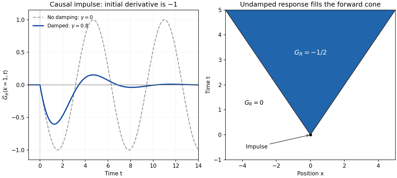
For $0<k^2<4/{\gamma }^2$, defineThe simple poles are ${\omega }_{\pm }=\pm {\Omega }_k-i{a}_k$. In the inverse transform $\tilde{G}(k,t)=\int e^{-i\omega t}\hat{G}d\omega /(2\pi )$, close the contour below for $t>0$. Its clockwise orientation gives $-i$ times the sum of residues. That sum isFor $t<0$, close above; there are no poles. The residue theorem therefore givesHere $\Theta$ is the Heaviside step function. At $k=0$ the continuous retarded limit is $-t\Theta (t)$. At critical damping, ${\Omega }_k\to 0$ likewise replaces $\sin ({\Omega }_{k}t)/{\Omega }_k$ by $t$; beyond the stated oscillatory range an imaginary ${\Omega }_k$ converts it to a hyperbolic sine. These continuations retain decaying temporal exponents.

For each fixed $k$, taking $\gamma \to 0^{+}$ givesFor $t>0$, invert in space and set $s=kt$:The correctly normalized sinc function transform isFor instance, $\sin s/s=\frac{1}{2}{\int }_{-1}^1{e}^{isy}dy$, and Fourier inversion immediately gives the factor $\pi$. The PDF's prefactor $\sqrt{2/\pi }$ is inconsistent with its top hat of unit height; it would give height $\sqrt{2\pi }$. Using the normalized identity yieldsas a distribution. The values assigned precisely at a wave front do not change that distribution. This is the negative of the standard one-dimensional retarded wave Green function, because the PDF's differential operator is $-{\partial }_t^2+{\partial }_x^2$.

The sign and initial data can be checked without any contour calculation. Integrating the spatial-Fourier equation through the impulse givesIn real space these are $G_R(x,0^{+})=0$ and ${\partial }_t{G}_R(x,0^{+})=-\delta (x)$. In particular,for a smooth test function $f$, confirming the negative delta-function initial velocity. Before the impulse the displacement and velocity are zero. The disturbance fills the forward causal cone for the constant-speed wave equation, whose fronts move at unit speed, consistent with $\rho =\kappa =1$. The final question's printed $\rho =k$ is interpreted as $\rho =\kappa$, referring to the elastic constant, not to the Fourier wavevector. No initial conditions were otherwise specified, so the causal choice has been made explicitly.

With the PDF's inverse Fourier transform convention, the derivatives act asso its forced differential operator becomes ${\omega }^2-k^2+i\gamma \omega k^2$. ThusFor the physical impulse response choose the retarded fundamental solution, vanishing before $t=0$. For $k\ne 0$ and $\gamma >0$, its poles lie in the lower half-plane. The retarded Fourier pole prescription $\omega \mapsto \omega +i0$ specifies the zero mode and the zero-damping limit as well; a Green function without a temporal or boundary prescription would otherwise permit homogeneous additions.

This is the Kelvin-Voigt rod Green function. Multiplying the homogeneous real-space equation by $-1$ givesA spatial Fourier mode therefore satisfies ${\ddot{\varphi }}_k+\gamma k^2{\dot{\varphi }}_k+k^2{\varphi }_k=0$: positive $\gamma$ really damps the motion. For sufficiently decaying fields its energy satisfiesThis checks the sign of the imaginary term in $\hat{G}$ independently of the transform calculation.

Use $x^{\mu }=(t,x)$ and Minkowski metric ${\eta }^{\mu \nu }=\mathrm{diag}(1,-1)$, with the wave speed equal to one. Regarding $\varphi$ as a scalar field, the symmetric canonical stress-energy tensor isIt obeys ${\partial }_{\mu }{T}^{\mu \nu }=0$ on the wave equation. For a scalar field the intrinsic spin current vanishes. The total orbital Lorentz current and its integrated angular-momentum tensor areBecause there is only one spatial dimension, its only independent possibly nonzero component iswhere $P=\int pdx$. The corresponding flux is ${\mathcal{J}}^{101}=t\mathcal{E}-xp$. Symmetry and conservation of $T$ giveThus $J^{01}$ is conserved provided the boundary flux vanishes and the integrals exist. For example, localized wave packets on an infinite line have this property. One can also check directly that $d\int x\mathcal{E}dx/dt=P$, so the two terms in $J^{01}$ have cancelling derivatives.

The significance is the boost charge of a one-dimensional scalar field. There is no independent spatial rotation or ordinary spatial angular-momentum component in one dimension. Instead, the action has the mathematical Lorentz invariance of a massless wave field with invariant speed $c_s=1$, and $J^{01}$ generates its boost. Its conservation says that the center of energy moves uniformly. This is a symmetry of the ideal wave-field model, rather than an assertion of fundamental vacuum Lorentz symmetry for a material rod. Fixed boundaries can break it, and a general solution with nonvanishing boundary flux need not conserve the integrated charge.

The derivatives of the Lagrangian density are ${\mathcal{L}}_{\varphi }=0$, ${\mathcal{L}}_{{\varphi }_t}={\varphi }_t$, and ${\mathcal{L}}_{{\varphi }_x}=-{\varphi }_x$. The Euler-Lagrange field equation is thereforeThis is the one-dimensional wave equation with wave speed $c_s=\sqrt{\kappa /\rho }=1$. Both signs of propagation are allowed: $\varphi (x,t)=F(x-t)+H(x+t)$ for sufficiently regular profiles.