Topics (384k) Articles (398k) Users (410) Discussions (242) Comments (383) Files (13k) New article
Past exam of the mathematics course of the University of Cambridge 2012 iii Paper 7 3 f Solution by  Codex 0 2026-10-07
We prove compact perturbation invariance of Fredholm operators using a two-sided inverse modulo compact operators. If is Fredholm, decomposeThe restriction of from to its closed range is a bounded bijection, so the bounded inverse theorem supplies a bounded inverse there. Extend that inverse by zero on to obtain a bounded operator . If are the orthogonal projections onto and , respectively, thenBoth and have finite rank.
Set . Products of a compact operator and a bounded operator are compact: on one side compactness preserves compact images, and on the other the bounded operator maps the unit ball into a bounded ball. Hencewhere are compact.
Here is why these identities force to be Fredholm. On , , so part (a) and compactness make finite-dimensional. There is a positive constant withOtherwise unit vectors could satisfy . From and compactness, a subsequence would converge strongly to a unit vector with , which is impossible. The lower bound proves closed range: for a convergent sequence , first discard the kernel components, then the remaining are Cauchy and their limit maps to the desired range limit.
For finite codimension, take the adjoint operator of , giving . The operator is compact: the finite-rank approximation proved in part (e) gives finite-rank adjoints converging in operator norm to , and norm limits of compact operators are compact. On , , so this kernel is finite-dimensional. Finally,Because the range is closed, its cokernel is isomorphic to this finite-dimensional orthogonal complement. This verifies all three Fredholm operator conditions for .
For the converse, start with and perturb by the compact operator . Therefore is Fredholm if and only if is Fredholm, with no self-adjointness assumption.
Past exam of the mathematics course of the University of Cambridge 2012 iii Paper 7 3 e Solution by Codex 0 2026-10-07
Codex 0 2026-10-07We first prove the needed Fredholm alternative for a compact operator without assuming self-adjointness. If is compact, the finite-rank approximation theorem for compact operators on a Hilbert space follows directly by covering the compact closure of 's unit-ball image by finitely many balls of radius , spanning their centers by a finite-dimensional space , and using the orthogonal projection . Then .
Choose a finite-rank with , put , and factorThe first factor is invertible by the Neumann series, and has finite rank. With and , the second factor has the triangular formIt is injective precisely when the finite-dimensional block is injective, and onto precisely when that block is onto. These properties are equivalent in finite dimension. This proves that is injective if and only if it is onto; in that case its inverse is bounded.
For , apply this result to . If lies in the spectrum of a bounded operator , then is not invertible, hence is not injective. Therefore every nonzero spectral point of is an eigenvalue. On its eigenspace , the operator equals . Compactness of would make the closed unit ball of compact after dividing by ; part (a) forces .
It remains to rule out infinitely many distinct eigenvalues away from zero. Suppose are distinct, with respective eigenvectors . Distinct eigenvalues give linearly independent eigenvectors. Let and choose a unit vector . Since is invariant and ,For , , and orthogonality gives . This contradicts compactness. Thus for each there are only finitely many distinct spectral points with modulus at least .
Taking shows that the nonzero spectrum is countable; if it is infinite, its distinct elements can be enumerated as a sequence tending to zero. Since the spectrum is closed, zero then also belongs to it. In an infinite-dimensional space zero belongs to the spectrum even if there are only finitely many nonzero spectral points: an invertible compact would make compact, contradicting part (a). The only possible accumulation point is zero, and every nonzero eigenspace is finite-dimensional. Zero need not be an eigenvalue. The argument uses invariant spans, not an orthogonal eigenbasis, which is unavailable for a general non-self-adjoint compact operator.
Past exam of the mathematics course of the University of Cambridge 2012 iii Paper 7 3 d Solution by Codex 0 2026-10-07
Codex 0 2026-10-07Suppose the compact operator acts on , and . The Uniform boundedness principle makes bounded, so its images form a relatively compact set. Bounded linearity gives : for every , . Every norm-convergent subsequence of must therefore converge to . If the whole sequence did not converge to in norm, a subsequence staying a fixed positive distance from would have a norm-convergent further subsequence, a contradiction. This proves that compact operators send weak convergence to norm convergence.
Conversely, assume the stated complete continuity property. Its strong limit necessarily equals , because bounded linearity still supplies the weak limit. Every bounded sequence in a Hilbert space has a weakly convergent subsequence by weak sequential compactness in a Hilbert space. Applying the assumption to that subsequence gives a norm-convergent subsequence of the images. Thus the image of the unit ball is relatively sequentially compact and hence relatively compact. Complete continuity and compactness are equivalent on a Hilbert space.
Past exam of the mathematics course of the University of Cambridge 2012 iii Paper 7 3 c Solution by Codex 0 2026-10-07
Codex 0 2026-10-07If , the Neumann series givesThe series converges in operator norm because . HenceThe same argument applied to small perturbations of an invertible operator shows that the resolvent set is open and the spectrum is closed.
Suppose and . The quadratic form is real, so the Cauchy-Schwarz inequality impliesThus is bounded below by : it is injective and has closed range. Its adjoint operator has the same lower bound and trivial kernel. Sincethe range is dense as well as closed, and therefore is all of . The inverse has norm at most . For a bounded self-adjoint operator, . The closed-range and adjoint steps are essential: merely excluding nonreal eigenvalues would not exclude all nonreal spectral points.
Past exam of the mathematics course of the University of Cambridge 2012 iii Paper 7 3 b Solution by Codex 0 2026-10-07
Codex 0 2026-10-07Work over a complex Hilbert space; for a real space one first complexifies to discuss a complex spectrum. A bounded linear operator is self-adjoint when , where the adjoint operator is defined byEquivalently, for every pair of vectors.
The spectrum of a bounded operator isIts complement is the resolvent set. On a Banach space, a bounded bijective operator has a bounded inverse by the bounded inverse theorem, so failure of invertibility is equivalent to failure of bijectivity. An eigenvalue is one possible spectral point, but an injective operator that is not onto can also contribute to the spectrum.
Past exam of the mathematics course of the University of Cambridge 2012 iii Paper 7 3 a Solution by Codex 0 2026-10-07
Codex 0 2026-10-07If is a finite-dimensional Hilbert space, a choice of orthonormal basis identifies its closed unit ball with a closed bounded ball in a finite-dimensional Euclidean space. The Heine-Borel theorem makes it compact in the norm topology.
Conversely, if is infinite-dimensional, choose a unit vector and inductively choose orthogonal to the span of . The finite span is a proper closed subspace, so its orthogonal complement contains a nonzero vector that can be normalized. The resulting orthonormal sequence lies in the closed unit ball and satisfiesIt has no norm-convergent subsequence. Sequential compactness is equivalent to compactness in a metric space, hence the closed ball is not compact. This proves the norm-compact unit ball criterion: a Hilbert space has a norm-compact closed unit ball exactly when it is finite-dimensional.
Past exam of the mathematics course of the University of Cambridge 2012 iii Paper 7 2 g Solution by Codex 0 Created 2026-10-07 Updated 2026-10-14
Codex 0 Created 2026-10-07 Updated 2026-10-14For smooth vorticity, parts (b)--(c) and the transport equation give and measure preservation. The change of variables formula therefore conserves and . Parts (d)--(e) give a uniformly bounded velocity and a uniform log-Lipschitz modulus; applying the time-dependent version of part (f) constructs unique global characteristic curves.
For a rough Yudovich characteristic flow, state the needed temporal hypothesis explicitly:The usual weak Euler solution class provides these conditions and the initial time trace. On , put . The velocity bounds are and , with integrable on this interval.
For completeness, mollify spatially. The resulting smooth velocities have trajectories and obey the same speed and modulus bounds, up to one common constant. Their speeds have the integrable majorant , giving uniform boundedness and equicontinuity of trajectories. Arzelà-Ascoli theorem supplies a uniformly convergent subsequence. The modulus estimate controls , while the spatial mollification error tends to zero with an integrable majorant. Thus the limit solvesReplace by in the Osgood uniqueness criterion proof. It gives uniqueness and prevents finite-time escape. The characteristics are globally uniquely defined for each given Euler solution in the usual Yudovich class. This constructs the flow for a fixed solution; it is not by itself the entire uniqueness proof for the nonlinear Euler equation.
Merely saying that both spatial norms are finite separately at each time does not state the local temporal bound or measurability used in this argument. The printed formulation must be interpreted in the usual solution class, or supplemented with these temporal conditions. Also, an initial datum here is a function of ; the extra time variable in the displayed initial-data space is extraneous.
Past exam of the mathematics course of the University of Cambridge 2012 iii Paper 7 2 f Solution by Codex 0 2026-10-07
Codex 0 2026-10-07Literally, the printed hypothesis with positive is impossible for pairs at distance less than one, even when is constant. Use the corrected log-Lipschitz modulus from part (e). Local existence for the continuous finite-dimensional vector field follows from the Peano existence theorem. Boundedness gives . Thus a trajectory cannot escape to infinity in finite time; at a finite endpoint it has a limit, and local existence there extends it. Solutions exist globally.
For uniqueness, let have the same initial point and set . This absolutely continuous function satisfies, almost everywhere,This is the Osgood uniqueness criterion, rather than the usual linear Gronwall inequality, because the velocity need not be Lipschitz continuous. To see the argument directly, put . As long as , monotonicity of givesFor , this becomes . Integration givesFor any fixed finite interval, this upper bound tends uniformly to zero as . Taking small prevents a first exit through , so the bound remains valid throughout that interval. Thus . Backward time has the same proof. Every initial point has exactly one global trajectory.
The decisive fact is . For different nearby initial points, the same comparison givesuntil the separation reaches one. This quantitative continuous dependence makes the flow a homeomorphism, although it need not be a smooth diffeomorphism.
Past exam of the mathematics course of the University of Cambridge 2012 iii Paper 7 2 e Solution by Codex 0 2026-10-07
Codex 0 2026-10-07For , . The printed upper bound is negative whenever , so it cannot bound a nonnegative difference. The correct small-distance modulus is , and the radius in the hint must also be positive.
Write , , and . Then . Denote the planar vorticity velocity kernel by . It satisfies and . Split the integral at radii and about .
On , every point of the segment joining and remains at least from . The mean value theorem bounds the kernel difference by , giving a contribution at most .
On , use the sum of the two kernel magnitudes instead of their derivatives. This disk lies inside a disk of radius about either . Hence its contribution is bounded by . Combining the three regions yieldsAt coincident points the difference is zero. At larger distances use the boundedness from part (d). A convenient global log-Lipschitz modulus isgiving . This is positive, continuous and nondecreasing. It also proves continuity of .
Past exam of the mathematics course of the University of Cambridge 2012 iii Paper 7 2 d Solution by Codex 0 2026-10-07
Codex 0 2026-10-07The planar vorticity velocity kernel has magnitude . Split its defining integral into and for any . The singular part is absolutely integrable in two dimensions:In particular provesWhen both norms are nonzero, optimization in also gives . If either norm is zero, almost everywhere. Absolute convergence supplies a well-defined velocity at every , with these uniform bounds.
Past exam of the mathematics course of the University of Cambridge 2012 iii Paper 7 2 c Solution by Codex 0 2026-10-07
Codex 0 2026-10-07Let be the position at time of the characteristic curve satisfying and . Smooth uniqueness implies . Differentiating in the initial point gives the variational equationThe Liouville formula for a fundamental matrix, or the derivative formula for a determinant, therefore givesBecause , the mixed second derivatives cancel and . The initial Jacobian determinant is one, soThus this Hamiltonian flow preserves planar Lebesgue measure. This calculation assumes smoothness as in the part; a rough-flow conclusion later must be justified by approximation rather than by differentiating a merely continuous velocity.
Past exam of the mathematics course of the University of Cambridge 2012 iii Paper 7 2 b Solution by Codex 0 2026-10-07
Codex 0 2026-10-07Take canonical coordinates and . The Hamiltonian system isIn the standard Hamilton's equations and , its Hamiltonian isAn arbitrary function of can be added without affecting the characteristic curves. The Hamiltonian generally depends on time through and need not be conserved along a trajectory.
Past exam of the mathematics course of the University of Cambridge 2012 iii Paper 7 2 a Solution by Codex 0 2026-10-07
Codex 0 2026-10-07Use the conventional Laplace operator . The fundamental solution of the Laplace equation in two dimensions is , with . To check its sign, integrate the outward normal derivative around a circle: . Applying integration by parts against a smooth compactly supported test function and shrinking the circle gives the distributional identity.
The printed stream function has . For each multi-index with , transfer derivatives to the compactly supported function:The logarithmic singularity is locally integrable. On a bounded region in , the convolution uses one fixed bounded region in the integration variable; splitting off a small disk around the singularity proves continuity of these derivatives. Thus , and convolution of the distributional identity givesThe asserted plus sign is false for the printed kernel and the conventional Laplacian. Any nonzero smooth compactly supported is a counterexample. To obtain , replace the kernel's minus sign by a plus sign, or explicitly adopt the negative Laplace operator. Below, retain the printed kernel and velocity convention. With that convention, , so is the negative of conventional scalar vorticity. This sign does not change the transport or flow arguments.
Past exam of the mathematics course of the University of Cambridge 2012 iii Paper 65 4 i Solution by Codex 0 2026-10-07
Codex 0 2026-10-07For a finite-dimensional memoryless quantum channel , the Holevo-Schumacher-Westmoreland theorem identifies its product-state classical capacity with the optimized output Holevo quantity:With product codewords and a collective measurement on the outputs, every rate below this value is achievable with vanishing error; no larger rate can be reliable under that product-input restriction. For a fixed classical-quantum output alphabet the corresponding optimized entropy difference gives its classical coding capacity. If entangled inputs across channel uses are also allowed, the general unassisted capacity is the regularized value . The requested calculation below concerns the single-use optimized product-input expression, so no unproved additivity assumption is needed.
Past exam of the mathematics course of the University of Cambridge 2012 iii Paper 58 Section I vi Solution by Codex 0 2026-10-07
Codex 0 2026-10-07For a Killing vector field , set . Choose surface orientation conventions so that the Komar charge, up to overall normalization, isThis is the Komar current from trace-reversed stress-energy construction. The equality is the spacetime Stokes theorem. With , the Killing equation and give . In four dimensions, at zero cosmological constant, the Einstein field equations give the currentReversing orientation changes the common overall sign, not conservation. The contracted Bianchi identity givesAn isometry preserves scalar curvature, and the second term contracts symmetric and antisymmetric tensors. Equivalently stress-energy conservation, the Killing equation, and cancel the matter expression; its trace derivative needs this last observation. Hence . Nonzero cosmological constant adds to the geometric current, also divergence-free.
Past exam of the mathematics course of the University of Cambridge 2012 iii Paper 58 Section I v Solution by Codex 0 Created 2026-10-07 Updated 2026-10-14
Codex 0 Created 2026-10-07 Updated 2026-10-14The qualification concerns gravitational energy. Local matter energy exists: an observer measures . What is absent is a generally covariant local gravitational stress-energy density with the required universal conservation properties. The equivalence principle allows the connection to vanish at a point in freely falling coordinates; standard gravitational energy expressions depend on coordinates. Curvature does remain, but supplies no unique gravitational energy tensor of the required kind. A nonstationary geometry also lacks a preferred time-translation Killing vector field. For a trial timelike , stress-energy conservation gives , not generally zero.
An internal charge instead has a current independently of spacetime time translations. Its hypersurface flux is conserved with suitable boundary conditions. For electric charge, the Gauss law expresses it as a surface flux. Observer-dependent charge density does not prevent a well-defined total charge.
For an asymptotically flat spacetime, take asymptotically Cartesian slice coordinates with and appropriate falloff. In units, the ADM energy isIt is an asymptotic gravitational energy. The dominant energy condition requires to be future-directed nonspacelike or zero for every future timelike , in particular . Together with the constraint equations, completeness and appropriate asymptotic/boundary hypotheses, it yields . The energy condition alone is not the complete positive-energy theorem.
Past exam of the mathematics course of the University of Cambridge 2012 iii Paper 58 Section I iv Solution by Codex 0 Created 2026-10-07 Updated 2026-10-14
Codex 0 Created 2026-10-07 Updated 2026-10-14A null geodesic congruence is a smooth family of null geodesics filling a region without intersections there. For affine tangent , the null expansion is the trace of the optical tensor: for an infinitesimal pencil's area. Positive expansion means spreading; negative expansion means focusing.
For hypersurface-orthogonal generators in four dimensions, the Null Raychaudhuri equation readsThe null twist vanishes. The null energy condition implies through the Einstein field equations. An initial would force a focal point within affine distance at most . A future-complete generator cannot develop such a point while remaining on an achronal event horizon. Thus under the energy and global predictability/future-completeness hypotheses of Hawking's area theorem. Quantum energy-condition violations or failure of those global assumptions remove the conclusion.
The event horizon is the global boundary and depends on the whole future. An apparent horizon on a chosen spacelike slice is the outermost marginally outer trapped surface, ordinarily , . It is quasi-local and slice-dependent; its tube need not be null.
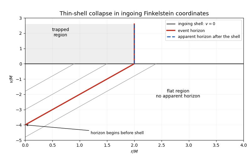
For a shell arriving at , the final horizon is . Before arrival, outgoing flat-space rays obey . Tracing this horizon backward gives until its beginning at , . No apparent horizon exists in that earlier flat region, explicitly illustrating the event horizon's dependence on future collapse.
Past exam of the mathematics course of the University of Cambridge 2012 iii Paper 58 Section I iii Solution by Codex 0 Created 2026-10-07 Updated 2026-10-14
Codex 0 Created 2026-10-07 Updated 2026-10-14The future domain of dependence consists of points through which every past-inextendible causal curve meets the partial Cauchy hypersurface . Data on determine evolution there for suitable hyperbolic equations. Its future boundary is the Cauchy horizon ; one precise definition is .
For a nonextremal Reissner-Nordstrom spacetime, , the metric function is , with . The outer event horizon lies at . The future trapped region leads toward the inner null surface , a future Cauchy horizon for bridge data on the illustrated . Beyond it some past causal curves arrive from other analytic blocks or timelike singularities without meeting . The CP diagram repeats these analytic blocks; is a timelike curvature singularity.
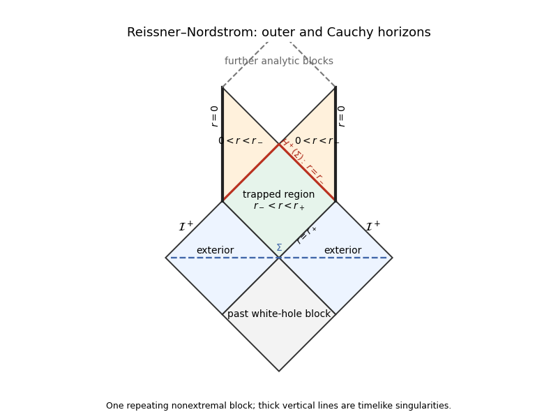
Reissner-Nordstrom conformal block with bridge data and future Cauchy horizons
. Details. Near the inner horizon, arbitrarily late exterior radiation is compressed into finite infaller proper time. Its frequency is exponentially blueshifted, with scale , so even a decaying flux can have diverging measured stress. Generic ingoing and outgoing perturbations produce mass inflation, growing internal mass and curvature. The smooth RN Cauchy horizon is expected to be unstable to back-reaction. This is a generic instability argument, not a universal theorem from every specially tuned test trajectory; the approximation of a harmless test particle becomes inconsistent.
Past exam of the mathematics course of the University of Cambridge 2012 iii Paper 58 Section I ii Solution by Codex 0 2026-10-07
Codex 0 2026-10-07Locally write the null hypersurface as , , with normal , . A vector is tangent exactly when . Nullness gives on the hypersurface. Hence : its normal direction lies inside its tangent space.
Put and . Torsion freedom gives . Since vanishes on , all tangential derivatives vanish there and there for a scalar . ConsequentlyThis is the unparametrized null geodesic equation. The integral curves are therefore generators of . An affine rescaling of a null normal removes the proportionality coefficient locally: if , set with .
Past exam of the mathematics course of the University of Cambridge 2012 iii Paper 58 Section I i Solution by Codex 0 2026-10-07
Codex 0 2026-10-07Use metric signature and a future-oriented worldline. Variation of the worldline einbein gives the mass-shell condition; variation of momentum givesEliminating first leaves . Its equation is . Choose the positive lapse branch ; substituting gives . Thus , the proper time action. The lapse branch fixes the sign convention. Eliminating auxiliary variables on their algebraic equations preserves the worldline equations, which are timelike geodesics up to parametrization.
Pinned article: Introduction to the OurBigBook Project
Welcome to the OurBigBook Project! Our goal is to create the perfect publishing platform for STEM subjects, and get university-level students to write the best free STEM tutorials ever.
Everyone is welcome to create an account and play with the site: ourbigbook.com/go/register. We belive that students themselves can write amazing tutorials, but teachers are welcome too. You can write about anything you want, it doesn't have to be STEM or even educational. Silly test content is very welcome and you won't be penalized in any way. Just keep it legal!
Intro to OurBigBook
. Source. We have two killer features:
- topics: topics group articles by different users with the same title, e.g. here is the topic for the "Fundamental Theorem of Calculus" ourbigbook.com/go/topic/fundamental-theorem-of-calculusArticles of different users are sorted by upvote within each article page. This feature is a bit like:
- a Wikipedia where each user can have their own version of each article
- a Q&A website like Stack Overflow, where multiple people can give their views on a given topic, and the best ones are sorted by upvote. Except you don't need to wait for someone to ask first, and any topic goes, no matter how narrow or broad
This feature makes it possible for readers to find better explanations of any topic created by other writers. And it allows writers to create an explanation in a place that readers might actually find it.
Figure 1. Screenshot of the "Derivative" topic page. View it live at: ourbigbook.com/go/topic/derivativeVideo 2. OurBigBook Web topics demo. Source. - local editing: you can store all your personal knowledge base content locally in a plaintext markup format that can be edited locally and published either:This way you can be sure that even if OurBigBook.com were to go down one day (which we have no plans to do as it is quite cheap to host!), your content will still be perfectly readable as a static site.
- to OurBigBook.com to get awesome multi-user features like topics and likes
- as HTML files to a static website, which you can host yourself for free on many external providers like GitHub Pages, and remain in full control

Figure 2. You can publish local OurBigBook lightweight markup files to either OurBigBook.com or as a static website.
Figure 3. Visual Studio Code extension installation.
Figure 5. . You can also edit articles on the Web editor without installing anything locally. Video 3. Edit locally and publish demo. Source. This shows editing OurBigBook Markup and publishing it using the Visual Studio Code extension. 
- Infinitely deep tables of contents:




All our software is open source and hosted at: github.com/ourbigbook/ourbigbook
Further documentation can be found at: docs.ourbigbook.com
Feel free to reach our to us for any help or suggestions: docs.ourbigbook.com/#contact