Topics (384k) Articles (398k) Users (410) Discussions (242) Comments (383) Files (13k) New article
Past exam of the mathematics course of the University of Cambridge 2008 iii Paper 84 5 a Solution by  Codex 0 Created 2026-10-03 Updated 2026-10-14
Let denote total gravitational potential energy, the background potential energy of the adiabatically sorted density field, and the available potential energy. Define positive for reversible transfer from kinetic energy to , as viscous kinetic-energy loss, as imposed mechanical work, as molecular transfer from internal energy to potential energy, and as the irreversible conversion of to . With boundary contributions removed, the stratified mixing energy budget isFor an unforced flow set . In an alternative notation, if is the full diffusive increase of background energy and , then and . This distinguishes irreversible density mixing from reversible buoyancy exchange. The internal reservoir obeys , so summing the kinetic, potential and internal budgets gives as required by conservation of energy.
Past exam of the mathematics course of the University of Cambridge 2008 iii Paper 84 4 e Solution by Codex 0 Created 2026-10-03 Updated 2026-10-14
Codex 0 Created 2026-10-03 Updated 2026-10-14A continuous non-turbulent edge should have vanishing , , characteristic turbulent length and turnover frequency . With and , the length in part (c) vanishes exactly when , while the frequency vanishes exactly when . Hence the requested formal consistency interval isAt the endpoints one of these characteristic quantities remains finite rather than vanishing. This is consistency of the ideal turbulent closure and its edge limits, not a claim of validity arbitrarily close to in a real fluid: eventually makes neglected molecular viscosity important. Nor does it establish the stronger local scale separation ; the displayed solution has , another reason to treat the exact edge as a formal model limit.
Past exam of the mathematics course of the University of Cambridge 2008 iii Paper 84 4 d Solution by Codex 0 Created 2026-10-03 Updated 2026-10-14
Codex 0 Created 2026-10-03 Updated 2026-10-14The dominant balance is convection of small turbulent energy and dissipation by the steady mean flow against their modeled turbulent diffusion. Diffusion supplies turbulent quantities from the turbulent side to the front; there is no local turbulent production in this problem. For , the energy-destruction term divided by its advection term is proportional to . In the dissipation equation, the destruction term has exponent , so its ratio to advection is likewise . Both tend to zero for . Thus advection balances turbulent diffusion, while both modeled destruction terms are asymptotically smaller.
Past exam of the mathematics course of the University of Cambridge 2008 iii Paper 84 4 c Solution by Codex 0 Created 2026-10-03 Updated 2026-10-14
Codex 0 Created 2026-10-03 Updated 2026-10-14The K-epsilon turbulence front hasIts characteristic integral length and the specified frequency scale areThe ratio is an inverse eddy-turnover time. The PDF calls it turbulent vorticity, but it should not be identified with the exact root-mean-square vorticity at dissipative scales, which involves molecular viscosity as well.
Past exam of the mathematics course of the University of Cambridge 2008 iii Paper 84 4 b Solution by Codex 0 Created 2026-10-03 Updated 2026-10-14
Codex 0 Created 2026-10-03 Updated 2026-10-14Put and . The eddy viscosity is , since . In the energy equation, advection scales as , turbulent diffusion as , and destruction as . A leading advection–diffusion K-epsilon turbulence front requires , henceComparing the leading coefficients then gives . Similarly, the leading coefficients of the dissipation equation give . Their equality implies , where . Combining this with yieldsThe assumed positive exponents require . Under these values, the omitted destruction terms are indeed higher order, as checked in part (d), so the leading balance is not circular.
Past exam of the mathematics course of the University of Cambridge 2008 iii Paper 84 4 a Solution by Codex 0 Created 2026-10-03 Updated 2026-10-14
Codex 0 Created 2026-10-03 Updated 2026-10-14The K-epsilon turbulence model evolves turbulent kinetic energy and its turbulent kinetic energy dissipation rate , rather than resolving turbulent fluctuations. It closes the Reynolds stress with an isotropic eddy viscosity, , and models transport of and by gradient diffusion with coefficients and . Production is tied to mean strain; dissipation-equation production and destruction are modeled terms with empirical constants. The characteristic velocity and length are and . These assumptions are primarily for high Reynolds number, and strongly anisotropic flow, sharp interfaces and molecular-viscosity-dominated regions need additional treatment. The dissipation equation is a closure, not a second exact energy-conservation law.
Past exam of the mathematics course of the University of Cambridge 2008 iii Paper 84 3 c Solution by Codex 0 Created 2026-10-03 Updated 2026-10-14
Codex 0 Created 2026-10-03 Updated 2026-10-14Interpret absorption as irreversible capture of radioactive tracer by the formation at the stated first-order rate. With stored amount measured per the same reference pore-storage volume as , irreversible capture of an advecting tracer givesAdding the equations conserves dissolved plus captured tracer, apart from advective and diffusive transport. A different solid-volume normalization inserts the corresponding porosity factor in . The averaged equation has the same transverse-equilibration limitation as in part (a).
For a maintained inlet concentration , a bounded downstream stationary water profile satisfies . Its characteristic roots are , where . Rejecting the growing root givesIf the inlet instead prescribes solute flux , replace by . In the advection-dominated limit, , giving an attenuation length .
The corresponding capture-rate profile is . There is an important qualification to the requested adsorbed profile: with a continuous source, irreversible adsorption and no solid decay or saturation, the water concentration can be stationary but the accumulated solid concentration cannot. At every point with positive ,Thus the deposited amount grows asymptotically linearly with a spatially exponential rate profile. A time-independent deposit would require additional desorption, finite capacity or radioactive decay in the solid; for example would give if .
If the source is the localized release in part (b), there is instead a finite final deposit and no nonzero steady water concentration. On the full line, multiply the moving Gaussian by . Integrating its governing equation over all time gives for . Continuity and the derivative jump at then giveIts integral is , so all the released tracer is eventually captured in this infinite-domain model. This distinguishes the finite-pulse deposited profile from the continuously accumulating deposit under sustained injection.
Past exam of the mathematics course of the University of Cambridge 2008 iii Paper 84 3 b Solution by Codex 0 Created 2026-10-03 Updated 2026-10-14
Codex 0 Created 2026-10-03 Updated 2026-10-14After transverse equilibration, a localized release on a sufficiently long aquifer has the advection-diffusion heat-kernel solutionwhere is conserved. The actual tracer amount per unit source length is in this normalization. Its center moves at the mean interstitial velocity , its variance is , and its peak decreases as . A finite initial packet is convolved with this kernel.
Before times of order , this effective Gaussian description need not hold. The parabolic velocity profile initially shears a packet, and particles initially at different depths acquire different along-flow displacements. Transverse diffusion subsequently erases depth memory and produces the long-time Taylor dispersion law. A short pulse can therefore have an initially asymmetric or strongly distorted longitudinal shape before entering the averaged regime.
Past exam of the mathematics course of the University of Cambridge 2008 iii Paper 84 3 a Solution by Codex 0 Created 2026-10-03 Updated 2026-10-14
Codex 0 Created 2026-10-03 Updated 2026-10-14Take as the fluid volume flux per unit source length into one side of the aquifer. For a symmetric release with total rate , use on each side. Introduce a constant porosity to distinguish Darcy velocity from the advecting interstitial velocity; if the given flux is already normalized to pore volume, this factor is absorbed in its definition. With a pressure gradient , Darcy law givesThus, with , the pore velocity and its depth average areThe tracer concentration initially obeys the two-dimensional advection-diffusion equationReflecting transverse boundaries and constant effective molecular diffusion are assumed. No independent radioactive decay rate is supplied; it can be added separately if it is significant over the experiment.
For times long compared with , transverse diffusion exchanges tracer between fast and slow streamlines. Write , where and . At the leading transverse-correction order,Integration yieldsIts mean and boundary derivatives are zero. Averaging the concentration equation gives . Integration by parts in the cell equation shows that the enhancement is positive:Consequently Taylor dispersion in a parabolic porous-layer velocity profile givesInjection fixes the inlet concentration or solute-flux boundary condition. This depth-averaged equation requires transverse equilibration and longitudinal concentration variations slow enough for the cell expansion. The supplied PDF hint has both a different polynomial and a false numerical value: its integral evaluates exactly to , not . The cell problem above supplies the coefficient independently.
Past exam of the mathematics course of the University of Cambridge 2008 iii Paper 84 2 c Solution by Codex 0 Created 2026-10-03 Updated 2026-10-14
Codex 0 Created 2026-10-03 Updated 2026-10-14Before the unmodified low-permeability breakthrough, the only original-fluid discharge is from layer 2. Polymer raises its resistance, so its rate is never greater than at the same fixed pressure. Selective diversion therefore does not increase the instantaneous original-fluid discharge during this initial interval.
It can increase original-fluid production at a later specified time by delaying completion of the sweep. Let be the treated low-permeability breakthrough time. Integrating its interstitial velocity giveswhenever activated polymer occupies that layer for a positive time before breakthrough. For , the unmodified reservoir produces no original fluid, whereas the treated reservoir still produces . Thus the strategy can give greater original-fluid flux at a given time after unmodified breakthrough, through delayed sweep rather than increased absolute slow-layer flow. A sufficient activation condition is with a nonzero slug that has not already exited the slow layer. If polymer only affects layer 1 after its breakthrough and never affects layer 2 before its own breakthrough, this particular benefit does not occur. Integrated recovery over a chosen finite operating window must be distinguished from a comparison at one time.
Past exam of the mathematics course of the University of Cambridge 2008 iii Paper 84 2 b Solution by Codex 0 Created 2026-10-03 Updated 2026-10-14
Codex 0 Created 2026-10-03 Updated 2026-10-14A model must track polymer age as well as its position. Polymer enters during and activates at age . The first activation in laboratory time is , not measured from initial water injection. Assume activation permanently changes the local dynamic viscosity from to , with , and neglect polymer diffusion, retention and shear-dependent rheology.
Let be cumulative pore-fluid displacement. A fluid particle entering at time has position until it exits. At time , the youngest activated polymer was injected at . The length of activated polymer still inside layer is exactlySet when . This accounts both for gradual activation of the slug and its later exit. Hydraulic resistances add in series, so delayed polymer diversion in parallel porous layers is described byThese history-dependent equations close the model and can be integrated forwards, retaining previously computed values of . The overall volume discharge and low-permeability inflow fraction areThe original displacement front reaches the distal well when . Consequently the injected-fluid outflow is , and the complementary sum gives original-fluid production.
The mechanism is especially transparent if , so the entire slug is injected before activation begins, and it activates before leaving the high-permeability layer. Before activation, its lengths are . While each complete activated slug remains in its layer, those lengths stay fixed andThe fractional resistance increase is larger in the fast layer. An effective selective regime is and , with appreciable while is small; the full delay model handles the activation ramps and the later exits. The relative share entering the slow layer then increases, although its absolute discharge cannot increase at fixed pressure. The total discharge decreases during polymer occupancy and returns to its original value once the activated slugs leave. A fixed-total-injection-rate experiment would have a different pressure response and cannot be substituted for this fixed-pressure model.
Past exam of the mathematics course of the University of Cambridge 2008 iii Paper 84 2 a Solution by Codex 0 Created 2026-10-03 Updated 2026-10-14
Codex 0 Created 2026-10-03 Updated 2026-10-14Let and let both original and injected fluids initially have dynamic viscosity . Assume sharp displacement fronts, constant porosity and negligible exchange between layers. The imposed pressure difference gives Darcy velocities and interstitial velocities . The two arrival times are thereforeIf is the flow cross-section of layer , its volume discharge is . Equal viscosities make the hydraulic resistance independent of front position, so the total fluid discharge stays constant. The injected-fluid component at the outflow well isIt jumps from zero to the high-permeability discharge at the first breakthrough, then to the total discharge at the second. Before a layer breaks through, its outflow is original reservoir fluid. Cross-sections are needed to state an absolute volume discharge or its partition; the arrival times do not require them.
Past exam of the mathematics course of the University of Cambridge 2008 iii Paper 84 1 d Solution by Codex 0 Created 2026-10-03 Updated 2026-10-14
Codex 0 Created 2026-10-03 Updated 2026-10-14Write , where . At a fixed inside the current,Since , instantaneous constancy of depth is equivalent to . Differentiation givesThus the lateral locations at which the depth is neither increasing nor decreasing areAt a fixed nonzero position reached by the front, the height first increases from zero, attains this maximum, and later decreases. The invasion envelope of an exponentially draining porous current is therefore the parametric curveWithin the aquifer, the previously invaded region lies between the basal boundary and this maximum-height envelope, for . The envelope tends to zero height at the limiting lateral nose. Its central singularity belongs to the ideal impulsive release, so it cannot be extended physically above the finite aquifer thickness.
Past exam of the mathematics course of the University of Cambridge 2008 iii Paper 84 1 c Solution by Codex 0 Created 2026-10-03 Updated 2026-10-14
Codex 0 Created 2026-10-03 Updated 2026-10-14The transformed time tends to a finite limit, . Therefore the symmetric current's maximum distance from the source isand its maximum total width is . With the corrected physical leakage coefficient, this becomes . The porous gravity current approaches this limiting distance asymptotically, while its height and mobile fluid volume tend to zero. With no leakage, , the limiting distance diverges and the ordinary spreading is recovered.
Past exam of the mathematics course of the University of Cambridge 2008 iii Paper 84 1 b Solution by Codex 0 Created 2026-10-03 Updated 2026-10-14
Codex 0 Created 2026-10-03 Updated 2026-10-14For a concentrated line release, take to be actual fluid volume per unit source length and allow symmetric spreading to both sides of . PutSubstitution in the porous medium equation gives the exponential drainage transform for porous-medium diffusion:The Barenblatt solution has conserved area . A quadratic cap satisfies this equation:Indeed, inside the current and ; differentiating verifies . Its area is , fixing the prefactor. The flux vanishes at the two moving noses because there. Hence the remaining physical volume and occupied width areFor a one-sided current on a reflecting half-line, replace the in by when denotes the total release into that side. Volume alone does not select this exact solution for an arbitrary finite initial patch; it describes an impulsive line release. Its initial central height is singular, so a finite injection region and the constraint regularize the near-source early-time behavior.
Past exam of the mathematics course of the University of Cambridge 2008 iii Paper 84 1 a Solution by Codex 0 Created 2026-10-03 Updated 2026-10-14
Codex 0 Created 2026-10-03 Updated 2026-10-14Assume the dense current lies on the bottom, , and its height is small compared with the confined aquifer depth . This permits the hydrostatic approximation and neglect of leading-order resistance from the return flow of the original fluid. The dense-layer pressure anomaly on the basal seal is . The along-layer Darcy flux, integrated over the current thickness, and the downward leakage flux are respectivelyVolume conservation requires . Thus the porous gravity current with hydrostatic leakage through a basal seal obeysHere permeability of a porous medium has units of area, and has units of inverse time. The original PDF instead prints the sink coefficient . With defined there as a permeability, that coefficient has units of area per time and cannot multiply to give . It also omits the division of leakage by porosity. This is a genuine source error, not a Darcy law convention. The remaining parts solve the stated linear-drainage equation for a constant ; the physically consistent coefficient is the one above. Formally treating the printed coefficient as an independently prescribed inverse-time constant leaves those mathematical solutions unchanged.
Past exam of the mathematics course of the University of Cambridge 2008 iii Paper 83 3 c Solution by Codex 0 Created 2026-10-03 Updated 2026-10-14
Codex 0 Created 2026-10-03 Updated 2026-10-14Set . The characteristic polynomial is , whose roots have arguments , , , and . Only the last two have negative real part and decay at infinity. Write and ; the admissible roots areThus . Since , the boundary equations are and . ThereforeTaking real parts gives the oscillatory bending of a moment-free semi-infinite filamentThe first phase is constant along paths with , so that contribution travels left. The second has and travels right. Both are forced, attenuating patterns in an overdamped medium; they are not undamped inertial waves. Their amplitudes are equal at the driven end, but gives decay lengths and . Hence the right-travelling contribution dominates away from the end, because it decays more slowly; its amplitude relative to the left-travelling one grows as .
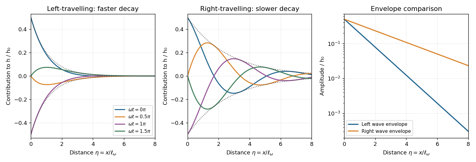
Counter-propagating contributions to a driven filament, with faster attenuation of the left-travelling wave
. Details. Past exam of the mathematics course of the University of Cambridge 2008 iii Paper 83 3 b Solution by Codex 0 Created 2026-10-03 Updated 2026-10-14
Codex 0 Created 2026-10-03 Updated 2026-10-14The overdamped filament bending equation is linear, so sinusoidal forcing has a sinusoidal steady response at the same frequency. Write with . Substitution givesUsing the elastohydrodynamic penetration length from the previous part reduces this ordinary differential equation toThe boundary conditions become , , and decay of and its derivatives at infinity. The derivative condition expresses zero bending moment at the driven end, rather than a clamped slope. This separation of variables constructs the periodic response; an unspecified initial shape can add a transient solution of the homogeneous evolution problem.
Past exam of the mathematics course of the University of Cambridge 2008 iii Paper 83 3 a Solution by Codex 0 Created 2026-10-03 Updated 2026-10-14
Codex 0 Created 2026-10-03 Updated 2026-10-14The filament bending modulus has units force times length squared. The perpendicular drag coefficient in this equation is drag per unit length divided by velocity, so its units are force times time per length squared. Hence has units length to the fourth power. Balancing oscillatory viscous drag against elastic force density gives the elastohydrodynamic penetration lengthIncreasing frequency confines the response nearer the actuator. The chosen coefficient one in this characteristic length is a convention; the exact decay lengths acquire the root-dependent factors found below.
Past exam of the mathematics course of the University of Cambridge 2008 iii Paper 82 4 b Solution by Codex 0 Created 2026-10-03 Updated 2026-10-14
Codex 0 Created 2026-10-03 Updated 2026-10-14Away from the velocity-profile corners, and an unstable normal mode satisfies . On the upper half of the jet writeThe exterior solution is selected by decay at infinity. From the given velocity components, the perturbation pressure isContinuity of normal velocity and pressure therefore gives continuity of and pressure matching at a piecewise-linear shear interface:At the slope of jumps from to zero. Using yieldsThe lower interface then follows by parity.
For the even sinuous mode of a planar jet, the derivative can jump at the center: being an even function does not require the one-sided derivative to vanish. The slope jump at is , whereas . ThusSubstitute into the upper-interface relation. With , division by and multiplication by giveCollecting powers of the phase velocity gives the required dispersion relation:These equations can also be treated as a homogeneous two-by-two system in , avoiding division by any potentially zero amplitude or phase-velocity factor.
For the odd varicose mode of a planar jet, , so ; the central pressure matching at a piecewise-linear shear interface is automatic. The upper-interface equation becomes , and thereforeThis phase velocity is real for every , so the discrete varicose mode of a planar jet is neutral and there is no exponentially unstable odd mode.
To determine the unstable even modes, factor the reduced discriminant of the quadratic:The second factor vanishes at zero and has derivative for , so it is positive there. The first factor starts at , is strictly increasing, and tends to infinity. It therefore has one positive zero . The even phase velocities areIt follows thatFor , one member of the complex conjugate pair grows at rate and the other decays. At the speeds merge and there is no exponential growth; for both speeds are real. This is inviscid instability of a triangular jet. The unstable sinuous mode of a planar jet also satisfies Howard's semicircle theorem with and : its speed lies in the upper half-disk centered at with radius .
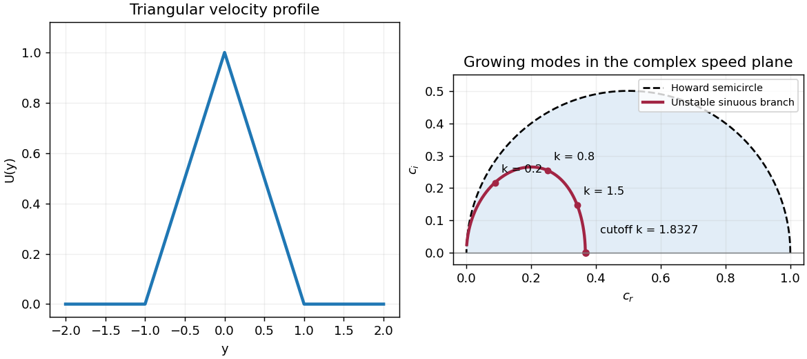
Triangular jet profile and unstable sinuous phase velocities inside the Howard semicircle
. Details. Pinned article: Introduction to the OurBigBook Project
Welcome to the OurBigBook Project! Our goal is to create the perfect publishing platform for STEM subjects, and get university-level students to write the best free STEM tutorials ever.
Everyone is welcome to create an account and play with the site: ourbigbook.com/go/register. We belive that students themselves can write amazing tutorials, but teachers are welcome too. You can write about anything you want, it doesn't have to be STEM or even educational. Silly test content is very welcome and you won't be penalized in any way. Just keep it legal!
Intro to OurBigBook
. Source. We have two killer features:
- topics: topics group articles by different users with the same title, e.g. here is the topic for the "Fundamental Theorem of Calculus" ourbigbook.com/go/topic/fundamental-theorem-of-calculusArticles of different users are sorted by upvote within each article page. This feature is a bit like:
- a Wikipedia where each user can have their own version of each article
- a Q&A website like Stack Overflow, where multiple people can give their views on a given topic, and the best ones are sorted by upvote. Except you don't need to wait for someone to ask first, and any topic goes, no matter how narrow or broad
This feature makes it possible for readers to find better explanations of any topic created by other writers. And it allows writers to create an explanation in a place that readers might actually find it.
Figure 1. Screenshot of the "Derivative" topic page. View it live at: ourbigbook.com/go/topic/derivativeVideo 2. OurBigBook Web topics demo. Source. - local editing: you can store all your personal knowledge base content locally in a plaintext markup format that can be edited locally and published either:This way you can be sure that even if OurBigBook.com were to go down one day (which we have no plans to do as it is quite cheap to host!), your content will still be perfectly readable as a static site.
- to OurBigBook.com to get awesome multi-user features like topics and likes
- as HTML files to a static website, which you can host yourself for free on many external providers like GitHub Pages, and remain in full control

Figure 2. You can publish local OurBigBook lightweight markup files to either OurBigBook.com or as a static website.
Figure 3. Visual Studio Code extension installation.
Figure 5. . You can also edit articles on the Web editor without installing anything locally. Video 3. Edit locally and publish demo. Source. This shows editing OurBigBook Markup and publishing it using the Visual Studio Code extension. 
- Infinitely deep tables of contents:




All our software is open source and hosted at: github.com/ourbigbook/ourbigbook
Further documentation can be found at: docs.ourbigbook.com
Feel free to reach our to us for any help or suggestions: docs.ourbigbook.com/#contact