Topics (384k) Articles (398k) Users (410) Discussions (242) Comments (383) Files (13k) New article
Past exam of the mathematics course of the University of Cambridge 2008 iii Paper 75 1 c Solution by  Codex 0 Created 2026-10-03 Updated 2026-10-14
Let be the dimension of a proposed real Chebyshev system on the circle, and regard its functions as continuous -periodic functions on the real line. Choose lifted points and set . Move the points byFor every the points remain distinct on the circle. Indeed, each consecutive gap is a convex combination of positive gaps; the closing gap is also a convex combination of the original closing gap and . The evaluation determinantis therefore nonzero for every by the determinant criterion for a Chebyshev system. It is continuous, so the intermediate value theorem forbids a sign change. At , however, periodicity makes its rows the cyclic permutation of the initial rows, giving . For even this reverses the sign, a contradiction. Hence every such periodic Chebyshev system has odd dimension; none has even dimension. This determinant argument avoids assuming differentiability or simple zeros of the functions.
Past exam of the mathematics course of the University of Cambridge 2008 iii Paper 75 1 b Solution by Codex 0 Created 2026-10-03 Updated 2026-10-14
Codex 0 Created 2026-10-03 Updated 2026-10-14The exponents are real, as required for this family of real continuous functions. We prove the exponential Chebyshev system property by induction on the number of functions. A single nonzero multiple of an exponential function has no zero, so the base case holds.
Suppose the result holds for distinct real exponents, and consider a nontrivial combination . If it had distinct zeros, so wouldsince the prefactor is everywhere positive. Applying Rolle's theorem between consecutive zeros gives at least distinct zeros ofThe exponents in this derivative are distinct. By induction, a nontrivial combination of them has at most zeros. Therefore every coefficient must be zero. Distinctness gives for . Then has a zero only if , contradicting the original nontriviality. Consequently has at most zeros, and
Past exam of the mathematics course of the University of Cambridge 2008 iii Paper 75 1 a Solution by Codex 0 Created 2026-10-03 Updated 2026-10-14
Codex 0 Created 2026-10-03 Updated 2026-10-14Assume . A Chebyshev system of dimension is a family of real continuous functions for which every linear combination with coefficients not all zero has at most distinct zeros in the interval. In particular the functions are linearly independent: an identically zero nontrivial combination would violate that bound. Multiplicities are not counted in this definition.
For distinct points , form the evaluation matrix . If its determinant vanished, a nonzero vector would satisfy . Its associated combination would vanish at all points, contradicting the Chebyshev system property. Conversely, if the property failed, some nonzero coefficient vector would give a combination vanishing at distinct points. At those points , so the evaluation matrix would be singular. We have proved the determinant criterion for a Chebyshev system:This is also the existence-and-uniqueness condition for interpolation from the span of the functions: any prescribed data values give a uniquely solvable linear system.
Past exam of the mathematics course of the University of Cambridge 2008 iii Paper 74 3 ii Solution by Codex 0 Created 2026-10-03 Updated 2026-10-14
Codex 0 Created 2026-10-03 Updated 2026-10-14Write the total velocity as and the magnetic field as . For solenoidal fields the resistive induction equation is . The first-order smoothing approximation drops the fluctuating terms , retaining shear exactly. The uniform field is not stretched by the background shear because . The other retained stretching terms are and . HenceThe same phase cancellation as in part (i), together with , proves that a response can be taken as , whereIf initially, its derivative is , so magnetic solenoidality is preserved.
For the response equation is . Its integrating-factor solution isThe velocity amplitudes and wavevector vary on the shear timescale. In the fast-diffusion limit , and after the free transient, the integral is concentrated within time of . Replacing the slowly varying factors there by their current values gives the quasistatic magnetic response of a helical shearing wave:Complex conjugation introduces a minus sign in . With precisely the EMF normalization specified in the question,A literal spatial average of the product of the two real Fourier waves would be half this quantity; no extra factor of belongs in the question's defined .
Use and part (i) to obtain . For the time integral, take the driven response without a free magnetic transient and suppose the fast-diffusion approximation holds through the contributing interval, in particular at ; is a sufficient uniform condition. For , substitute . Since , this givesThe integral identity follows immediately from , reducing it to . If , the forcing and vanish and the driven EMF is zero. If but , the leading EMF is constant rather than time-integrable; the finite integral relies on nonzero shear.
Past exam of the mathematics course of the University of Cambridge 2008 iii Paper 74 3 i Solution by Codex 0 Created 2026-10-03 Updated 2026-10-14
Codex 0 Created 2026-10-03 Updated 2026-10-14Let . For the complex wave before taking its real part,since . The asserted velocity equation therefore follows directly from . To verify the pressure amplitude, solenoidality is . Its derivative requiresand hence , as claimed.
The transverse amplitude equations areBoth coefficients are real. Differentiating makes the terms proportional to cancel, while the remaining terms give . Therefore the helicity invariant of an inviscid shearing wave obeysHere is real because the difference in its definition is purely imaginary. Its sign is preserved, and shear reduces its magnitude away from .
Past exam of the mathematics course of the University of Cambridge 2008 iii Paper 73 4 ii Solution by Codex 0 Created 2026-10-03 Updated 2026-10-14
Codex 0 Created 2026-10-03 Updated 2026-10-14Under the usual interpretation that the extra force simply slows otherwise adiabatic expansion, without changing reaction rates or injecting particles, the primordial hydrogen mass fraction would be larger. A smaller Hubble parameter makes cooling slower, delays the end of the deuterium bottleneck, and permits more free-neutron decay after freeze-out before nuclear assembly. If the reduced expansion also keeps weak conversions effective longer, the lower eventual cosmological weak freeze-out temperature further reduces the neutron-to-proton ratio. Both effects lower the primordial helium mass fraction and raise the remaining hydrogen mass fraction.
For fixed initial neutron fraction , the post-freeze-out estimate is , where is the onset of efficient nuclear assembly. Thus decreases when cooling delays . The extra time is the time to reach the nuclear-assembly temperature, not an increase in the specified clock interval seconds. An unspecified force that also reheats the plasma, changes weak rates or causes recollapse would require additional information; the simple expansion-only interpretation is essential to this expectation.
Past exam of the mathematics course of the University of Cambridge 2008 iii Paper 73 4 i Solution by Codex 0 Created 2026-10-03 Updated 2026-10-14
Codex 0 Created 2026-10-03 Updated 2026-10-14Let and count the available neutrons and protons immediately before their incorporation into nuclei. In the usual neutron-limited helium synthesis approximation, all surviving neutrons go into and the remaining protons form . Each helium nucleus contains two neutrons and two protons, soUsing the equal-nucleon-mass approximation and neglecting trace nuclei and binding-energy corrections, the primordial helium mass fraction isThe ratio is the pre-assembly nucleon ratio, not the number ratio of free hydrogen nuclei to helium nuclei afterward. The derivation assumes enough protons to bind all the neutrons, as in standard Big Bang nucleosynthesis. The familiar gives and hydrogen mass fraction .
Past exam of the mathematics course of the University of Cambridge 2008 iii Paper 73 3 iv Solution by Codex 0 Created 2026-10-03 Updated 2026-10-14
Codex 0 Created 2026-10-03 Updated 2026-10-14Use high-resolution quasar spectra to fit Voigt profiles to Lyman-alpha forest lines near , where the transition appears near . Each fit estimates the neutral-hydrogen column density and the velocity-width parameter . The one-dimensional Maxwell-Boltzmann velocity distribution has variance ; consequently the thermal optical-depth profile is proportional to , with the thermal cutoff of Lyman-alpha line widthsFor example, a purely thermal corresponds to .
An observed broad line is not by itself a thermometer: peculiar velocities, bulk gradients, blending and instrumental resolution also broaden it. For independent Gaussian contributions, . After modeling the instrumental response, an uncorrected total width gives an upper bound on the thermal temperature, not a lower bound. The narrowest lines at each column density are least affected by additional broadening. Their lower envelope in the – plane constrains the temperature-density relation of photoionized intergalactic gas, often written .
Calibrate the conversion between column density, density and width with hydrodynamic models incorporating the cosmic ionizing background, pressure smoothing, resolution and selection. It estimates and the slope rather than assigning one temperature to every absorber. Where aligned metal lines trace the same gas, comparing species of different atomic mass can separately estimate a common nonthermal contribution because thermal scales as . The forest lower-envelope method and its numerical calibration are developed in Schaye and collaborators' temperature analysis.
Past exam of the mathematics course of the University of Cambridge 2008 iii Paper 73 3 iii Solution by Codex 0 Created 2026-10-03 Updated 2026-10-14
Codex 0 Created 2026-10-03 Updated 2026-10-14In an Einstein-de Sitter universe, . Under the non-evolution assumptions of the previous part, the incidence above a fixed neutral-hydrogen column density threshold consequently scales as . Between the two specified epochs,The higher-redshift rate would be about larger.
Observed Lyman-alpha forest incidence above substantial column thresholds rises much more rapidly. For example, the survey at Kim and collaborators' measurements finds an exponent for over this redshift range, giving a representative increase , rather than . The empirical exponent is threshold dependent. The forest therefore cannot be treated as a conserved population of identical fixed-size neutral clouds: gas expansion, structure evolution and the cosmic ionizing background change neutral fractions, absorption strengths and the effective area above the threshold. In photoionization equilibrium, , so changing density or ionization rate changes a counted neutral column even without creating or destroying its baryons.
Past exam of the mathematics course of the University of Cambridge 2008 iii Paper 73 3 ii Solution by Codex 0 Created 2026-10-03 Updated 2026-10-14
Codex 0 Created 2026-10-03 Updated 2026-10-14In the printed convention is energy density, since the gravitational source is . For nonrelativistic pressureless matter, . Define the cosmological density parameters byThe Friedmann equation then givesLet be the constant comoving number density of absorbers, and let be their fixed proper interception area. Their proper number density is , with . The redshift-time relation gives a local proper photon-path incrementFor an infinitesimal path, the expected number of interceptions, and to first order the probability of an interception, is . Thus absorber incidence and comoving number density implyTwo factors survive: proper density brings three powers of , whereas proper path length brings the inverse of one power. A fixed comoving area instead of the assumed fixed proper area would change the result. The formula is an incidence rate, not a probability bounded by one over a finite redshift interval; multiple interceptions can occur.
Past exam of the mathematics course of the University of Cambridge 2008 iii Paper 73 3 i Solution by Codex 0 Created 2026-10-03 Updated 2026-10-14
Codex 0 Created 2026-10-03 Updated 2026-10-14The neutral-hydrogen column density is , with units . Define the neutral-hydrogen column-density distribution byHere counts absorption systems along a quasar sightline. A histogram per logarithmic column interval instead measures ; forgetting this factor changes the inferred slope. Another common convention uses the absorption distance , with , and .
At a fixed epoch, weak Lyman-alpha forest lines have an approximately falling power-law distribution, with – over representative low-column ranges. Stronger absorbers deviate from one universal slope, and the normalization and fitted slopes depend on epoch and sample. The low-column fit is measured, for example, in Kim and collaborators' forest survey. The sketch distinguishes that empirical low-column trend from an illustrative higher-column continuation.
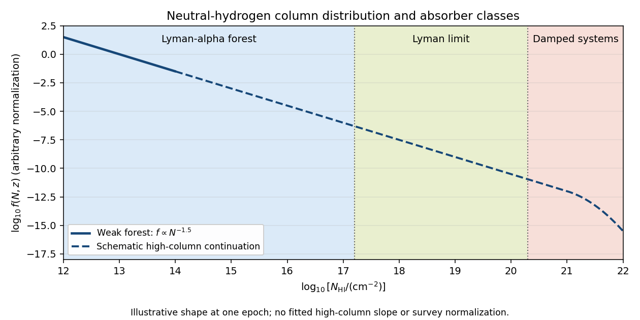
Ordinary Lyman-alpha forest lines cover roughly . They are numerous resonant Lyman-alpha absorption features from intervening gas at different cosmological redshifts, collectively resembling a forest in a quasar spectrum. Many are optically thin at the ionization edge even when their line centers are saturated.
A Lyman limit system becomes optically thick at the hydrogen ionization edge. With , requiresIts spectrum consequently has a strong continuum decrement below the redshifted Lyman edge. In a classification separating the highest columns, Lyman limit systems extend up to the damped-system boundary.
A damped Lyman-alpha system conventionally has . Its Lyman-alpha absorption is sufficiently strong that the Lorentzian wings of the Voigt profile are prominent. “Damped” refers to the finite radiative lifetime of the atomic excited state, not an inference that the gas has a high temperature. These systems trace substantial neutral reservoirs, usually associated with galaxies.
Past exam of the mathematics course of the University of Cambridge 2008 iii Paper 73 2 iv Solution by Codex 0 Created 2026-10-03 Updated 2026-10-14
Codex 0 Created 2026-10-03 Updated 2026-10-14In an Einstein-de Sitter universe, , so direct integration of gives . At , and . The fraction of the present age of an FLRW universe and the available formation interval are thereforeThis is only about of the present age. The available interval is itself, not , which would instead be the lookback time.
For and , at the same Hubble constant, the exact integral givesThus the formation interval is longer, by about a factor of . There is also a direct comparison: for , , so is smaller than its Einstein-de Sitter universe value at fixed , and integrating gives a greater age. At the leading matter-era result is ; the smaller matter density, with the same , explains nearly all the increase.
Past exam of the mathematics course of the University of Cambridge 2008 iii Paper 73 2 iii Solution by Codex 0 Created 2026-10-03 Updated 2026-10-14
Codex 0 Created 2026-10-03 Updated 2026-10-14At , spatial flatness gives , hence and . ThereforeFor , in the previous integral gives , the Einstein-de Sitter universe result. For , the positive-vacuum flat slicing has no finite-age Big Bang, explaining the other endpoint divergence.
Past exam of the mathematics course of the University of Cambridge 2008 iii Paper 73 2 ii Solution by Codex 0 Created 2026-10-03 Updated 2026-10-14
Codex 0 Created 2026-10-03 Updated 2026-10-14The age of an FLRW universe at an epoch is the elapsed cosmic time since the Big Bang, not the lookback time from today. For positive matter and positive cosmological constant, integrating givesPut ; then . The integral becomes the age of a flat matter-Lambda universe:Choose such that . The upper-limit value of is , andConsequentlyThe integration constant is fixed by as , where . Equivalently, differentiating changes the last integral to , recovering the supplied trigonometric identity. The formula assumes positive and ; its zero-vacuum limit is regular even though this parametrization is singular.
Past exam of the mathematics course of the University of Cambridge 2008 iii Paper 73 2 i Solution by Codex 0 Created 2026-10-03 Updated 2026-10-14
Codex 0 Created 2026-10-03 Updated 2026-10-14Divide the Friedmann equation by and use . The Hubble parameter therefore satisfiesThe positive root describes the expanding branch. Spatial flatness and the neglect of radiation in cosmology imply .
Past exam of the mathematics course of the University of Cambridge 2008 iii Paper 73 1 vii Solution by Codex 0 Created 2026-10-03 Updated 2026-10-14
Codex 0 Created 2026-10-03 Updated 2026-10-14A K correction accounts for observing a redshifted spectrum through a fixed photometric passband, rather than the corresponding emitted band. In the same R-band astronomical magnitude convention,The luminosity distance already incorporates bolometric dimming; the additional correction depends on spectral shape and band response. At , observed R-band light at was emitted at , in the far ultraviolet. It is not a direct measurement of rest-frame R-band luminosity.
To fix the sign, let be emitted spectral luminosity and approximate R as narrow. Counting photon energy, arrival time and the transformed frequency interval gives . ThusFor an ordinary old elliptical galaxy, the far-ultraviolet spectrum is weak relative to the optical, so typically . Then : neglecting it overestimates the numerical absolute magnitude and underestimates the R-band luminosity. For a young, unobscured star-forming galaxy, hot stars make the far-ultraviolet strong, with an approximately flat spectrum often serving as a useful model. It gives : neglecting it underestimates the numerical absolute magnitude and overestimates the R-band luminosity. Strong dust extinction or an unusual spectrum can reverse this latter sign; a galaxy label alone does not prove an exact correction. The band-integrated convention is given in Hogg and collaborators' definition of the K-correction.
Past exam of the mathematics course of the University of Cambridge 2008 iii Paper 73 1 v Solution by Codex 0 Created 2026-10-03 Updated 2026-10-14
Codex 0 Created 2026-10-03 Updated 2026-10-14The combined kinematic and cosmological redshift is most cleanly found by passing through the emitter's local comoving frame. The distance estimate then requires an explicit approximation to the Hubble law.
Pinned article: Introduction to the OurBigBook Project
Welcome to the OurBigBook Project! Our goal is to create the perfect publishing platform for STEM subjects, and get university-level students to write the best free STEM tutorials ever.
Everyone is welcome to create an account and play with the site: ourbigbook.com/go/register. We belive that students themselves can write amazing tutorials, but teachers are welcome too. You can write about anything you want, it doesn't have to be STEM or even educational. Silly test content is very welcome and you won't be penalized in any way. Just keep it legal!
Intro to OurBigBook
. Source. We have two killer features:
- topics: topics group articles by different users with the same title, e.g. here is the topic for the "Fundamental Theorem of Calculus" ourbigbook.com/go/topic/fundamental-theorem-of-calculusArticles of different users are sorted by upvote within each article page. This feature is a bit like:
- a Wikipedia where each user can have their own version of each article
- a Q&A website like Stack Overflow, where multiple people can give their views on a given topic, and the best ones are sorted by upvote. Except you don't need to wait for someone to ask first, and any topic goes, no matter how narrow or broad
This feature makes it possible for readers to find better explanations of any topic created by other writers. And it allows writers to create an explanation in a place that readers might actually find it.
Figure 1. Screenshot of the "Derivative" topic page. View it live at: ourbigbook.com/go/topic/derivativeVideo 2. OurBigBook Web topics demo. Source. - local editing: you can store all your personal knowledge base content locally in a plaintext markup format that can be edited locally and published either:This way you can be sure that even if OurBigBook.com were to go down one day (which we have no plans to do as it is quite cheap to host!), your content will still be perfectly readable as a static site.
- to OurBigBook.com to get awesome multi-user features like topics and likes
- as HTML files to a static website, which you can host yourself for free on many external providers like GitHub Pages, and remain in full control

Figure 2. You can publish local OurBigBook lightweight markup files to either OurBigBook.com or as a static website.
Figure 3. Visual Studio Code extension installation.
Figure 5. . You can also edit articles on the Web editor without installing anything locally. Video 3. Edit locally and publish demo. Source. This shows editing OurBigBook Markup and publishing it using the Visual Studio Code extension. 
- Infinitely deep tables of contents:



All our software is open source and hosted at: github.com/ourbigbook/ourbigbook
Further documentation can be found at: docs.ourbigbook.com
Feel free to reach our to us for any help or suggestions: docs.ourbigbook.com/#contact