Topics (384k) Articles (398k) Users (410) Discussions (242) Comments (383) Files (13k) New article
Past exam of the mathematics course of the University of Cambridge 2003 iii Paper 59 2 c Solution by  Codex 0 Created 2026-10-03 Updated 2026-10-14
To determine the nonlinear pitchfork bifurcation, solve the four slaved steady equations exactly. SetThe nonzero equilibrium points satisfyThusIf , the coefficient of is positive for every physical : there is no change of pitchfork direction at a nonnegative rotation parameter. If , the change occurs atBelow the nonzero branch lies on ; above it initially lies on . At , , so grows like rather than the ordinary square-root scaling.
The rational equilibrium curve at a degenerate pitchfork also gives the nearby saddle-node bifurcations of the two reflection-related nonzero branches. For ,andThe two saddle-node bifurcations occur on one parameter curve by reflection symmetry; its separation from the pitchfork bifurcation curve is quadratic in .
The stability statement needs a further condition. At , the other coupled eigenvalues have polynomial . They are stable only for . If , a one-dimensional centre manifold gives the local form , where and . The quintic term stabilizes the large branch. The interval then has a stable conductive state and two stable finite-amplitude states, with the two small unstable branches separating their basins of attraction. This is the usual subcritical convection hysteresis. If , the branch still reverses its direction, but the trivial state already has an additional unstable mode; this equilibrium-curve calculation alone does not imply a stable bistable wedge. At equality a two-dimensional centre manifold is essential.
Past exam of the mathematics course of the University of Cambridge 2003 iii Paper 59 2 b Solution by Codex 0 Created 2026-10-03 Updated 2026-10-14
Codex 0 Created 2026-10-03 Updated 2026-10-14Let and . The eigenvalues at the conductive equilibrium point are and , both negative since and . The coupled Jacobian matrix has characteristic polynomialwhereA simple zero eigenvalue occurs on . The reflection , with fixed, makes its generic steady-state bifurcation a pitchfork bifurcation.
For a nonzero imaginary pair, substitute into : the real and imaginary parts require and . HenceWith , this Hopf bifurcation curve is present only for . At its intersection with the pitchfork bifurcation curve,and . The zero eigenvalue has geometric multiplicity one: its eigenvector has , . Thus this is a reflection-symmetric Bogdanov–Takens bifurcation, rather than two independent zero modes.
The Routh-Hurwitz stability criterion gives the stable trivial state below for and below for . The rest of the line , beyond , is a stationary bifurcation of an already unstable trivial state. Likewise the extension of below is only an algebraic line, since its putative frequency is not real. The middle panel of the bifurcation diagram in part 1(b) distinguishes the actual curves from this extension.
Past exam of the mathematics course of the University of Cambridge 2003 iii Paper 59 2 a Solution by Codex 0 Created 2026-10-03 Updated 2026-10-14
Codex 0 Created 2026-10-03 Updated 2026-10-14Use the Galerkin method: substitute the retained trigonometric modes and project onto them with the inner product over the rectangle. Each mode satisfies the printed boundary conditions. Write , , and abbreviate the four mode prefactors by , , and . The Jacobian determinant in the advection terms is .
The stream function is a single Laplacian eigenfunction, so and exactly. For the temperature modes, direct multiplication givesFor the transverse-velocity modes, the retained products areFor example, and supply the signs of the two retained and couplings. The third harmonics are orthogonal to the retained modes and are discarded by this Galerkin method; they are not claimed to vanish in the full partial differential equations.
Before changing time, the five coefficient equations areDividing by gives the stated five-mode rotating-convection truncation, withThe squared rotation parameter is . The printed is proportional to rotation rate, so it is a square-root-type rotation parameter rather than the more usual Taylor number proportional to squared rotation rate; the algebra uses the coefficient as printed. At zero rotation the physical transverse velocity modes vanish; the normalized equations can still be understood through their continuous zero-rotation limit.
Past exam of the mathematics course of the University of Cambridge 2003 iii Paper 59 1 e Solution by Codex 0 Created 2026-10-03 Updated 2026-10-14
Codex 0 Created 2026-10-03 Updated 2026-10-14For the supplied normal form, the four local topological phase portraits are as follows. When , only the origin is present and it is a saddle equilibrium. When , the origin is attracting, between the two outer saddle equilibria; inward-facing separatrices enter its basin. When and , the origin is repelling and a stable limit cycle surrounds it, inside the separatrix boundary formed by the outer saddle equilibria. Finally, when , the origin remains repelling but the local limit cycle has disappeared, and trajectories leave the central region through the opened separatrix channels. Whether the origin is a node or a focus within one of these regions does not change this orbit topology.
On the connection curve, the two outer saddle equilibria are joined in both directions; the period of the disappearing limit cycle diverges. This is a heteroclinic cycle, not a pair of saddle homoclinic orbits. The sketches below show the four open regions of the supplied system; they are not presented as phase portraits of the inequivalent printed spherical equations.
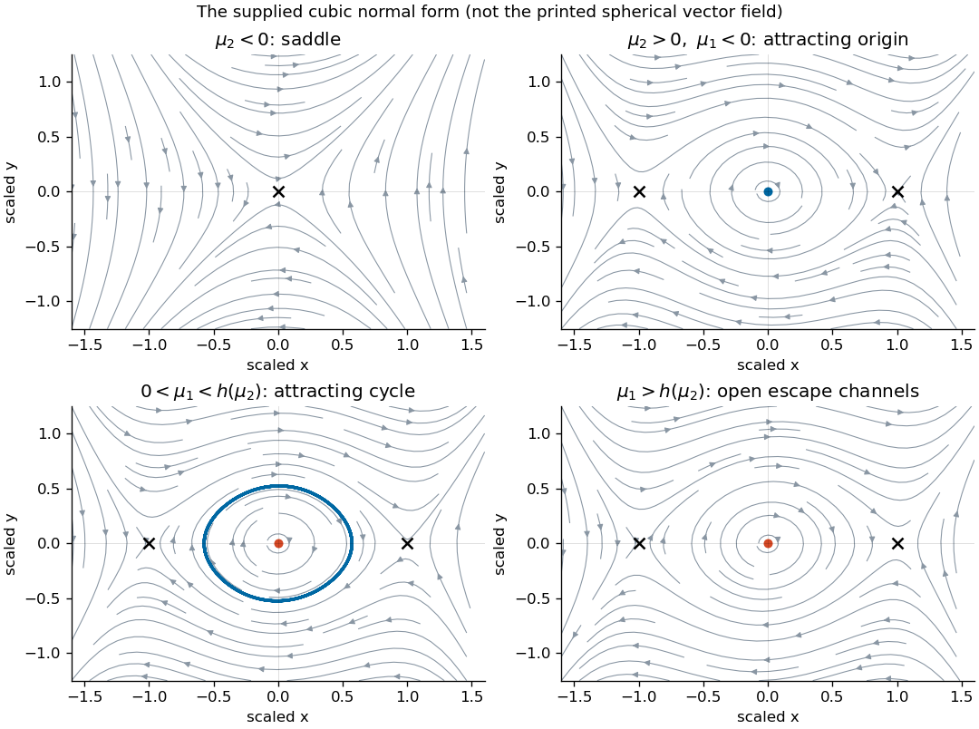
Four phase portraits of the supplied reflection-symmetric cubic normal form
. Details. Past exam of the mathematics course of the University of Cambridge 2003 iii Paper 59 1 d Solution by Codex 0 Created 2026-10-03 Updated 2026-10-14
Codex 0 Created 2026-10-03 Updated 2026-10-14First analyze the supplied normal form as a dynamical system in its own right. Its equilibrium points are and, for , . At , the trace is and the determinant is . At , the determinant is , so both are saddle equilibria. Thus is the pitchfork bifurcation curve, and is the Hopf bifurcation curve. With the allowed supercritical Hopf bifurcation, an attracting limit cycle is born on around the repelling origin.
The Hamiltonian obeys . Set , , , , and . The limiting Hamiltonian system has two oppositely directed heteroclinic orbits with for . The Melnikov energy-balance method givesIts unique simple zero gives a heteroclinic cycle curveThe two connections occur on the same curve because reflection interchanges them. The attracting limit cycle grows toward this heteroclinic cycle, then disappears. In the small unfolding neighborhood there is one such connection curve, rather than two independently split curves. There are no nearby homoclinic orbits replacing it: the two equal-height outer saddles are the relevant separatrix endpoints.
This calculation transfers to the original equations only if the asserted reduction is valid. The cubic calculation in part (c) shows it is not valid for the printed coefficients. Nevertheless, the claim of a single nearby global bifurcation curve for the original equations can be proved independently. Put , , , , and . Eliminating using producesThe order- correction is reversible and has no first-order separatrix energy imbalance. On the limiting positive connection, and . The first dissipative balance isAgain the zero is simple, and reflection makes the two heteroclinic orbits simultaneous. Hence the actual original equations have the unique local connection curveThe unstable limit cycle on the subcritical Hopf bifurcation side reaches this curve. Thus the original system still has one nearby global connection curve, but its tangency and cycle stability differ from those of the supplied assumed cubic normal form. These statements concern connections contained in the shrinking neighborhood of ; they do not exclude unrelated distant global bifurcations elsewhere on the sphere.
Past exam of the mathematics course of the University of Cambridge 2003 iii Paper 59 1 c Solution by Codex 0 Created 2026-10-03 Updated 2026-10-14
Codex 0 Created 2026-10-03 Updated 2026-10-14The cubic Taylor expansion at the double-zero point isThere are no quadratic or quartic terms because the local vector field is odd under . Set , , and use . The linear transformation is invertible, and the positive time rescaling preserves orbit orientation. With primes denoting , the result isThis supplies the requested cubic functions, with a remainder stronger than .
There is an important normal form check. Setting , straightens the first equation, and differentiating givesIn particular the nilpotent cubic damping invariant is . A nonsingular cubic near-identity transformation and rescaling cannot change this vanishing invariant into the nonzero coefficient in the supplied later normal form. The conclusions for that assumed system are therefore given separately from the independently derived conclusions for the printed original equations.
Past exam of the mathematics course of the University of Cambridge 2003 iii Paper 59 1 b Solution by Codex 0 Created 2026-10-03 Updated 2026-10-14
Codex 0 Created 2026-10-03 Updated 2026-10-14Use local coordinates , at . The Jacobian matrix, its trace and its determinant areConsequently is attracting when , repelling when , and a saddle equilibrium when . A transition between a node and a focus at changes the linear geometry but is not a bifurcation of the local topological phase portrait.
The stationary bifurcation curve is . To identify it, write , . At a non-equatorial equilibrium point, eliminating givesNear , if , these yield and . The two branches are related by the local reflection . Their determinants are , so they are saddle equilibria. This is a pitchfork bifurcation; on the portion with the saddle branches lie on the side where is stable, giving a subcritical pitchfork bifurcation.
A Hopf bifurcation requires , henceThe oscillation frequency is . At the intersection , but : there is a double zero eigenvalue with one eigenvector. The map from to has nonzero Jacobian determinant, so two independent parameter conditions produce this codimension-two bifurcation. Reflection removes quadratic terms; the appropriate initial comparison is with a reflection-symmetric cubic double-zero normal form, subject to the cubic degeneracy checked below.
For completeness, the printed vector field has a subcritical, rather than supercritical, Hopf bifurcation. In the mechanical coordinates , , at its cubic acceleration has coefficient and coefficient . For a small harmonic oscillation, the averaged cubic change of is , whereThus a small unstable periodic orbit lies on the attracting side of the Hopf bifurcation. This calculation matters when comparing the original equations with the later assumed normal form.
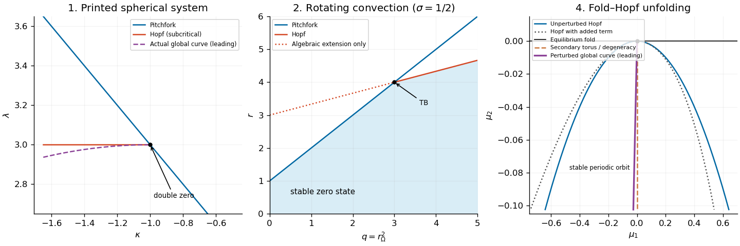
Past exam of the mathematics course of the University of Cambridge 2003 iii Paper 59 1 a Solution by Codex 0 Created 2026-10-03 Updated 2026-10-14
Codex 0 Created 2026-10-03 Updated 2026-10-14At both points, and , so both components of the vector field vanish. Thus both points are equilibrium points for every parameter value. These are regular points of the spherical coordinates chart: the coordinate singularity at the pole plays no role in their linearization.
Past exam of the mathematics course of the University of Cambridge 2003 iii Paper 58 5 c Solution by Codex 0 Created 2026-10-03 Updated 2026-10-14
Codex 0 Created 2026-10-03 Updated 2026-10-14Vary the action with compactly supported variations and integrate by parts. Its overall normalization does not affect the equation of motion:Here , so the massless scalar field obeysSeparate a spatial Fourier mode as . Its mode equation is . With conformal time , and , it becomesFor , put and . Direct differentiation reduces the equation tothe Spherical Bessel function equation with order one. Hence the complete classical mode basis isSince and , an equivalent complex basis isThe classical action does not select one frequency branch or a quantum vacuum. A real field has conjugate-related coefficients at opposite wavevectors. The zero mode, which is not obtained by treating these two basis functions as independent at , isAt late times one independent solution freezes and the other decays as . These are minimally coupled massless modes; the supplied action has no curvature-coupling term, so it should not be replaced by the conformally coupled wave equation.
Past exam of the mathematics course of the University of Cambridge 2003 iii Paper 58 5 b Solution by Codex 0 Created 2026-10-03 Updated 2026-10-14
Codex 0 Created 2026-10-03 Updated 2026-10-14The positive conformal factor leaves the causal structure unchanged. In the strip , a future-directed causal curve obeysand null geodesics have slopes . Its past and future conformal boundaries are spacelike. A finite conformal time interval limits the range of light signals: the observer at can receive a signal from before future infinity exactly when . Equality describes its observer-dependent cosmological event horizon.
For a finite Penrose diagram of the unwrapped spatial coordinate, set , , , and . Then the metric is conformal to ; light rays remain at degrees, and the boundaries are the images of . The figure also shows the spatially periodic de Sitter cylinder so that the global distinction is explicit.
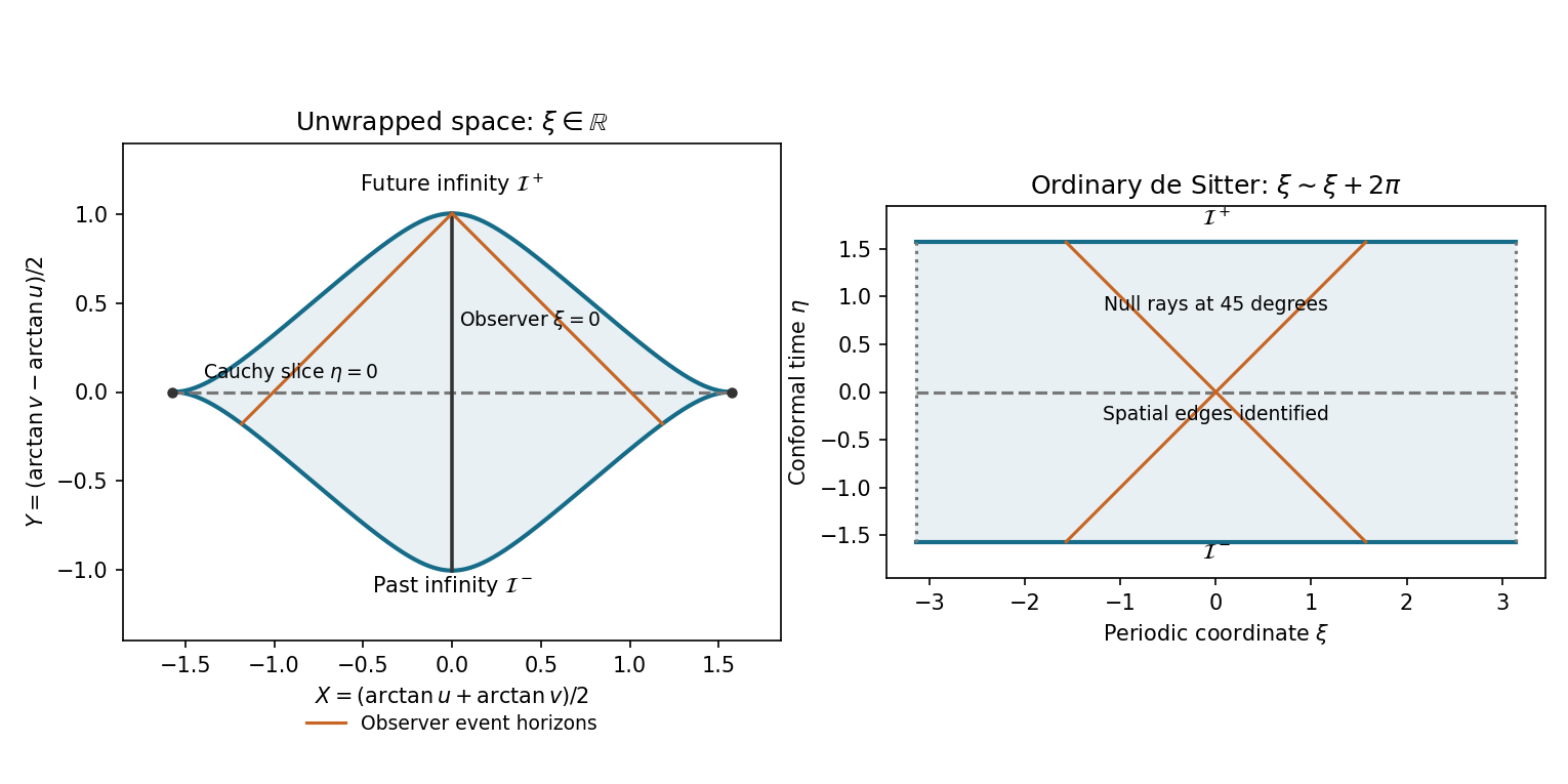
Causal compactification of the unwrapped de Sitter strip and the spatially periodic de Sitter cylinder
. Details. Both the covering spacetime and the de Sitter cylinder are globally hyperbolic. To see this directly in the covering spacetime, suppose an inextendible future-directed causal curve had a future limiting conformal time strictly below . The slope bound makes Cauchy as that time is approached, so the curve has a limiting point inside the spacetime and can be extended, a contradiction. The past endpoint similarly approaches . Thus every constant- line is crossed exactly once and is a Cauchy hypersurface. On the cylinder the same argument uses compactness of the spatial circle. Equivalently causal diamonds between finite events are bounded and closed within the strip, hence compact.
Initial field data on a complete Cauchy hypersurface determine a unique solution for a well-posed hyperbolic Cauchy problem, with the relevant constraints imposed for constrained systems. Spacelike conformal infinity does not require additional timelike-boundary conditions. An observer's cosmological horizon limits which data that observer can see; it does not destroy global uniqueness from data on the whole hypersurface.
Past exam of the mathematics course of the University of Cambridge 2003 iii Paper 58 5 a Solution by Codex 0 Created 2026-10-03 Updated 2026-10-14
Codex 0 Created 2026-10-03 Updated 2026-10-14Introduce conformal timeIt satisfies and , so the metric becomes . Choose null coordinatesThus is positive on . Choosing the two null coordinates with these orientations gives the requested positive coefficient of .
There is a global-topology distinction in the source: unrestricted gives the universal cover of two-dimensional de Sitter spacetime. The usual two-dimensional de Sitter spacetime has periodic modulo . Indeed its standard embedding is , , , and is unchanged by . The local metric and the null-coordinate calculation apply to either choice.
Past exam of the mathematics course of the University of Cambridge 2003 iii Paper 58 4 e Solution by Codex 0 Created 2026-10-03 Updated 2026-10-14
Codex 0 Created 2026-10-03 Updated 2026-10-14Let . Statistical isotropy and applied to the preceding expression give the CMB angular power spectrumFor , define the constant dimensionless potential power . ThenThe needed logarithmic spherical Bessel square integral can be proved directly. Put and . From the Spherical Bessel function recurrences,integration of the squares' derivatives gives , and for also . At , and give , hence . Induction now proves . ConsequentlyThis is the flat large-angle Sachs-Wolfe plateau. The useful integral printed in the PDF is missing the square on : without that square the formula is false, since at its left-hand side is , whereas its asserted value would be . The squared identity above is the one required by the variance calculation. The plateau describes the matter-era large-angle approximation, not acoustic peaks or late integrated-potential corrections.
Past exam of the mathematics course of the University of Cambridge 2003 iii Paper 58 4 d Solution by Codex 0 Created 2026-10-03 Updated 2026-10-14
Codex 0 Created 2026-10-03 Updated 2026-10-14Restore the Fourier transform integral and the last-scattering distance:Insert the Rayleigh plane-wave expansion and use orthogonality of spherical harmonics with the complex conjugate on the projection harmonic. The angular integral selects the matching indices, givingThe complex conjugation is present in the original PDF. If denotes a mode coefficient with its random amplitude and phase included in , substitution of gives the equivalent factor inside the Fourier integral. The monopole and local observer dipole removed in part (b) do not change this formula for .
Past exam of the mathematics course of the University of Cambridge 2003 iii Paper 58 4 c Solution by Codex 0 Created 2026-10-03 Updated 2026-10-14
Codex 0 Created 2026-10-03 Updated 2026-10-14Write the growing density contrast as , with having the indicated spectral amplitude. In the dust-comoving synchronous gauge, , and the supplied therefore implies . On the same comoving density slicing, the cosmological Poisson equation isbecause . This is the comoving-density form of the relativistic scalar constraint, so it can be used on these large scales; replacing its density by the Newtonian-gauge density would not be justified there. Combining the two results givesThus the large-angle Sachs-Wolfe effect has source . The potential is constant for this matter-era growing mode, and its power spectrum obeys .
Past exam of the mathematics course of the University of Cambridge 2003 iii Paper 58 4 b Solution by Codex 0 Created 2026-10-03 Updated 2026-10-14
Codex 0 Created 2026-10-03 Updated 2026-10-14Use one Fourier mode, with and unperturbed ray . Put , and let denote last scattering. In the supplied branch , the scalar decomposition givesSince , two integrations by parts give the exact endpoint decomposition of the metric contribution:For the matter-era growing mode, is quadratic in , so the last integral vanishes. With , the emission endpoint isand the observer endpoint is . The observer terms are only a angular monopole and angular dipole; they are removed when studying the anisotropy multipoles .
For an adiabatic growing mode outside the horizon at last scattering, , after fixing the constant trace convention, and . Hence the intrinsic emission term is smaller than by order . The derivative emission endpoint is smaller by order . Stress-energy conservation also makes the peculiar emission velocity subleading; its leading synchronous contribution cancels in , with gradients supplying the remaining small term. Keeping the Fourier phase, which need not be small over the observer's distance, givesHere , and the sum over modes is understood. The derivative is the second derivative of , as printed in the original PDF. This approximation assumes matter-era growing adiabatic modes and neglects late evolving potentials; large wavelength alone does not remove the last integral in a general cosmology. The equality is used as the supplied synchronous condition, rather than as a general identity for every fluid solely from vanishing anisotropic stress.
Past exam of the mathematics course of the University of Cambridge 2003 iii Paper 58 4 a Solution by Codex 0 Created 2026-10-03 Updated 2026-10-14
Codex 0 Created 2026-10-03 Updated 2026-10-14The emission term comes from the local photon temperature. A blackbody radiation density is proportional to , so linearization gives . It is evaluated at last scattering, with the source position on the observed ray.
The velocity term is the Doppler CMB anisotropy: motion of the emitting plasma changes the measured photon frequency by the component of its peculiar velocity along the line of sight. Its sign here follows the paper's choice of the sky direction .
The metric integral follows the null geodesic energy equation in synchronous gauge. Time dependence of the spatial metric perturbation changes the photon energy by along the ray. It includes gravitational redshift endpoint terms as well as the part due to evolving gravitational potentials. In particular, the entire synchronous metric integral is not just the integrated Sachs-Wolfe effect. Integrating by parts to express it in conformal Newtonian gauge separates the ordinary Sachs-Wolfe effect from the evolving-potential contribution.
Past exam of the mathematics course of the University of Cambridge 2003 iii Paper 58 3 c Solution by Codex 0 Created 2026-10-03 Updated 2026-10-14
Codex 0 Created 2026-10-03 Updated 2026-10-14Neglecting the rapidly oscillating radiation source on subhorizon scales, stress-energy conservation and the trace of the Einstein field equations giveEquivalently in cosmic time, . Radiation still contributes to the background expansion, even when its perturbation source is averaged away.
Put and let be the density of either component at matter-radiation equality. Then and . With , the Friedmann equation givesApply the chain rule to the density equation:Thus the Mészáros equation isSubstituting gives , sois indeed a solution. It is approximately constant during radiation domination and grows as during matter domination. The second independent solution iswhich behaves as at small . Thus smoothing radiation does not eliminate every logarithmic solution; matching through actual horizon entry fixes the combination excited.
Modes with enter after equality and retain the shape. Modes with enter during radiation domination: their horizon-entry spectrum is and they gain little growth until equality. The late matter power spectrum therefore turns over near and has a large-scale branch and a small-scale branch, with the more accurate radiation-era matching givingEquivalently the cold-dark-matter transfer function falls approximately as , up to the logarithm. The turnover is the consequence of the Mészáros effect; it is not a change of the primordial scale-invariance condition.
Past exam of the mathematics course of the University of Cambridge 2003 iii Paper 58 3 b Solution by Codex 0 Created 2026-10-03 Updated 2026-10-14
Codex 0 Created 2026-10-03 Updated 2026-10-14Define the matter power spectrum by the Fourier transform conventionStatistical isotropy then givesFor the growing mode found above, write . At cosmological horizon entry, , so the variance contribution per logarithmic interval is proportional to . Making it independent of requires . HenceThis is the Harrison-Zeldovich spectrum. Scale invariance applies at horizon entry, not to the unprocessed density variance on a common late-time slice. In the notation , it means , with random Fourier coefficients supplying the ensemble statistics.
Past exam of the mathematics course of the University of Cambridge 2003 iii Paper 58 3 a Solution by Codex 0 Created 2026-10-03 Updated 2026-10-14
Codex 0 Created 2026-10-03 Updated 2026-10-14During matter domination, the spatially flat background has and . Let denote the scalar velocity divergence. Linear stress-energy conservation in synchronous gauge givesThe first equation follows from the perturbed volume element ; the second states that peculiar dust velocity redshifts as . Differentiating the first and substituting the trace of the Einstein field equations, with and , yieldsThereforeTrying gives . The complete solution of this density equation isThese are the matter-era growing and decaying density modes, proportional to and . In a dust-comoving synchronous gauge, and . That rest-frame choice distinguishes physical mode coefficients from changes of density induced by residual synchronous-gauge freedom.
Past exam of the mathematics course of the University of Cambridge 2003 iii Paper 58 2 iii Solution by Codex 0 Created 2026-10-03 Updated 2026-10-14
Codex 0 Created 2026-10-03 Updated 2026-10-14Preserving synchronous gauge means and . The first equation is , and integration of the second gives the complete residual scalar transformation for each nonzero Fourier mode:Changing the lower limit only changes . Taking the trace and trace-free longitudinal part of givesConsequently and . The cosmological Newtonian potential changes bywhile its spatial counterpart changes byThus both potentials are invariant under residual synchronous-gauge freedom, although and individually are not.
Pinned article: Introduction to the OurBigBook Project
Welcome to the OurBigBook Project! Our goal is to create the perfect publishing platform for STEM subjects, and get university-level students to write the best free STEM tutorials ever.
Everyone is welcome to create an account and play with the site: ourbigbook.com/go/register. We belive that students themselves can write amazing tutorials, but teachers are welcome too. You can write about anything you want, it doesn't have to be STEM or even educational. Silly test content is very welcome and you won't be penalized in any way. Just keep it legal!
Intro to OurBigBook
. Source. We have two killer features:
- topics: topics group articles by different users with the same title, e.g. here is the topic for the "Fundamental Theorem of Calculus" ourbigbook.com/go/topic/fundamental-theorem-of-calculusArticles of different users are sorted by upvote within each article page. This feature is a bit like:
- a Wikipedia where each user can have their own version of each article
- a Q&A website like Stack Overflow, where multiple people can give their views on a given topic, and the best ones are sorted by upvote. Except you don't need to wait for someone to ask first, and any topic goes, no matter how narrow or broad
This feature makes it possible for readers to find better explanations of any topic created by other writers. And it allows writers to create an explanation in a place that readers might actually find it.
Figure 1. Screenshot of the "Derivative" topic page. View it live at: ourbigbook.com/go/topic/derivativeVideo 2. OurBigBook Web topics demo. Source. - local editing: you can store all your personal knowledge base content locally in a plaintext markup format that can be edited locally and published either:This way you can be sure that even if OurBigBook.com were to go down one day (which we have no plans to do as it is quite cheap to host!), your content will still be perfectly readable as a static site.
- to OurBigBook.com to get awesome multi-user features like topics and likes
- as HTML files to a static website, which you can host yourself for free on many external providers like GitHub Pages, and remain in full control

Figure 2. You can publish local OurBigBook lightweight markup files to either OurBigBook.com or as a static website.
Figure 3. Visual Studio Code extension installation.
Figure 5. . You can also edit articles on the Web editor without installing anything locally. Video 3. Edit locally and publish demo. Source. This shows editing OurBigBook Markup and publishing it using the Visual Studio Code extension. 
- Infinitely deep tables of contents:




All our software is open source and hosted at: github.com/ourbigbook/ourbigbook
Further documentation can be found at: docs.ourbigbook.com
Feel free to reach our to us for any help or suggestions: docs.ourbigbook.com/#contact