Topics (384k) Articles (398k) Users (410) Discussions (242) Comments (383) Files (13k) New article
Past exam of the mathematics course of the University of Cambridge 2003 iii Paper 65 2 i Solution by  Codex 0 Created 2026-10-03 Updated 2026-10-14
Assume an axisymmetric thin disk in the fixed Newtonian potential of a point mass, negligible disk self-gravity, and slow evolution compared with an orbital period. Radial pressure and radial inertia are small compared with gravity and centrifugal acceleration, so with , independent of height and time. Assume no mass loss or torque through the upper and lower disk faces. Define the surface density of a disk, mass-weighted radial velocity and integrated shear stress byVertical integration of the continuity equation givesThe azimuthal momentum equation, including the geometric term , gives conservation of angular momentum in terms of :Subtracting times mass conservation eliminates the time derivative and leaves .
Define the effective density-weighted viscosity of a disk through the actual stress:If the local viscous stress is , this reduces to . The definition can also describe an effective turbulent transport stress, provided the same shear closure is appropriate. Since , outward transport corresponds to and positive .
For Keplerian rotation, and . ThereforeSubstitution into mass conservation yields the Keplerian viscous diffusion equationThe absence of surface fluxes, fixed rotation law and leading thin-disk approximation are essential: a wind, appreciable radial inertia or evolving gravitational potential would alter this reduction.
Past exam of the mathematics course of the University of Cambridge 2003 iii Paper 65 1 iii Solution by Codex 0 Created 2026-10-03 Updated 2026-10-14
Codex 0 Created 2026-10-03 Updated 2026-10-14Let . Because the specific entropy is constant along the horizontal flow, the specific enthalpy identity gives . Dotting the ideal magnetohydrodynamic momentum equation with therefore givesOn the field-aligned horizontal branch, . Directly evaluating the horizontal components of the curl givesThe scalar triple-product identity consequently makes the magnetic work . Meanwhile . The previously established field-line constancy of now gives the planar ideal-MHD Bernoulli invariantThis is conservation of total energy transported along a magnetic field line, including electromagnetic work. To see its flux interpretation, the ideal magnetohydrodynamic energy conservation law has fluxThe second term is the Poynting vector, since . Substitution of givesThe steady divergence of this horizontal energy flux is zero. Magnetic stress can change the ordinary hydrodynamic quantity in the Bernoulli equation by doing work; the term accounts for the accompanying Poynting flux. When , the velocity is completely field-aligned, , and the usual hydrodynamic Bernoulli quantity is constant. These conclusions require the field-aligned branch and ; the arbitrary constant- flow from the first part is not covered by this particular invariant.
Past exam of the mathematics course of the University of Cambridge 2003 iii Paper 65 1 ii Solution by Codex 0 Created 2026-10-03 Updated 2026-10-14
Codex 0 Created 2026-10-03 Updated 2026-10-14Continue on the branch of steady planar ideal-MHD field-line invariants, with and positive . Adiabatic entropy transport gives . As all quantities are -independent,The axial component of the ideal magnetohydrodynamic momentum equation has no pressure or gravitational term. Magnetic tension givesSince is constant along a magnetic field line, this becomesSubtracting the two axial invariants yields the useful compatibility relationThe squared ratio of horizontal flow speed to horizontal Alfvén speed is ; vector equality with the horizontal Alfvén velocity additionally requires . If , the right side is a nonzero constant along the field line, so a regular finite cannot permit anywhere. This is the nondegenerate exclusion.
However, does not imply . The Alfvénic degeneracy of steady planar MHD is a genuine exception: take constant , , and a constant magnetic field with nonzero horizontal and axial components, and setEvery equation holds, but the horizontal velocity equals the horizontal Alfvén velocity everywhere despite . Therefore the printed pointwise exclusion needs a nondegeneracy hypothesis, such as . The general conclusion is the boxed compatibility relation; when , it says and allows the Alfvénic branch.
Past exam of the mathematics course of the University of Cambridge 2003 iii Paper 65 1 i Solution by Codex 0 Created 2026-10-03 Updated 2026-10-14
Codex 0 Created 2026-10-03 Updated 2026-10-14Write horizontal components with a subscript . The steady ideal magnetohydrodynamic induction equation gives . Since , its horizontal components implyThus is a spatial constant. A vanishing axial electric field, , is needed to infer horizontal alignment. It is satisfied, for example, if the constant electric field vanishes at a boundary or at infinity. With this additional condition and , define the magnetohydrodynamic mass loading by , and put . ThenThe steady continuity equation and the solenoidal magnetic-field constraint giveAlso . Using the vector identity for the curl of a cross product, together with and , its curl is . HenceThese are steady planar ideal-MHD field-line invariants: both quantities are constant along a magnetic field line.
The zero-electric-field condition does not follow from the printed stationarity assumptions alone. Constant , , and , with , satisfy every displayed ideal magnetohydrodynamics equation but have perpendicular horizontal velocity and magnetic field. Their is nonzero, so no give the stated decomposition. The field-line decomposition is valid on the branch; as an unrestricted implication, the first claim has this counterexample. The subsequent calculations use that branch.
Past exam of the mathematics course of the University of Cambridge 2003 iii Paper 63 4 d Solution by Codex 0 Created 2026-10-03 Updated 2026-10-14
Codex 0 Created 2026-10-03 Updated 2026-10-14An X-ray binary contains a compact accretor supplied by a donor star. Most bright systems contain a neutron star or black hole. Gas arrives by Roche-lobe overflow, a captured stellar wind, or donor outflows, commonly forming an accretion disk. The primary energy source is the release of gravitational binding energy during accretion, with a characteristic accretion luminosityFor a neutron star, can be near its material radius; for a black hole, radiation is produced by the flow outside the horizon. For and , , so accretion can release much more energy per unit mass than hydrogen burning. The hot inner flow, boundary layer or accretion column emits X-rays.
In a high-mass X-ray binary, a massive, relatively short-lived donor often supplies gas through a strong wind or an equatorial outflow; some systems instead undergo Roche-lobe overflow. These objects trace young stellar populations. In a low-mass X-ray binary, a lower-mass donor commonly fills its Roche lobe and feeds a disk. Such systems can persist in older populations. These mass labels refer to the donor, not the compact accretor.
A magnetized neutron star can channel accretion onto its poles, producing an accreting X-ray pulsar as the star rotates. Accretion transfers angular momentum, so changes in spin constrain the flow and magnetic coupling. A Type I X-ray burst has a different origin: accumulated hydrogen or helium undergoes unstable thermonuclear burning on a neutron star surface. It rises rapidly and then cools as the fuel is exhausted. A black hole has no material surface supporting the same surface-fuel mechanism.
Orbital motion and optical observations of the donor constrain masses, with inclination and donor-model uncertainties. A compact mass exceeding plausible stable neutron star masses supports a black hole interpretation. Rapid variability probes the small emitting region, while disk spectra and recurrent outbursts probe accretion and its instabilities. The Eddington luminosity,is obtained by balancing radiative acceleration against ; it is a useful luminosity scale under the assumed isotropic, opacity-controlled force law. Geometry and time dependence can complicate its application. X-ray binaries reveal compact stars through efficient gravitational accretion, with pulsations, bursts and orbital dynamics distinguishing their physical components.
Past exam of the mathematics course of the University of Cambridge 2003 iii Paper 63 4 c Solution by Codex 0 Created 2026-10-03 Updated 2026-10-14
Codex 0 Created 2026-10-03 Updated 2026-10-14A Type Ia supernova is a thermonuclear disruption associated with a carbon-oxygen white dwarf in a binary system. Electron degeneracy pressure supports the dense star, and initially depends much less on temperature than an ideal gas pressure does. Once carbon burning heats degenerate material, the immediate pressure response is insufficient to produce the usual expansion-and-cooling thermostat. The strongly temperature-sensitive nuclear reactions can therefore undergo a thermonuclear runaway.
One channel involves accretion toward the Chandrasekhar limit, about solar masses for a typical electron composition. Other proposed channels involve merging white dwarfs or an initial helium-layer detonation that triggers carbon burning below that mass. Thus the Chandrasekhar limit motivates an important model, but it is not an assumption that every Type Ia supernova has exactly the same progenitor mass or ignition history. Burning carbon and oxygen into more tightly bound nuclei releases enough nuclear binding energy to overcome the stellar gravitational binding energy. An ordinary successful event ejects the star rather than leaving the compact core characteristic of a core-collapse supernova.
The ejecta contain iron-group material, including radioactive nickel-56, and intermediate-mass elements from incomplete burning. The radioactively powered Type Ia supernova light curve is powered largely by the nickel-56 to cobalt-56 to iron-56 decay chain: its energetic products heat the ejecta, and radiative diffusion delays the emerging radiation. Near maximum light, ordinary Type Ia supernovae show prominent silicon absorption and lack the hydrogen lines defining Type II events. The spectral classification and the thermonuclear mechanism provide complementary descriptions.
The similar progenitors and radioactive power make Type Ia supernovae useful standard candles, but their peak luminosities are not identical. The relation between light curve width and peak brightness, together with color corrections, allows standardization for distance measurements. Extinction, composition and explosion diversity still introduce systematic uncertainties. A Type Ia event is a white-dwarf thermonuclear explosion with a radioactively powered light curve; its corrected luminosity makes it a valuable distance indicator.
Past exam of the mathematics course of the University of Cambridge 2003 iii Paper 63 4 b Solution by Codex 0 Created 2026-10-03 Updated 2026-10-14
Codex 0 Created 2026-10-03 Updated 2026-10-14The first argument is the energy budget. The gravitational energy reservoir is of order , so the Kelvin-Helmholtz cooling time is . For the Sun, , and give years. This is much shorter than the approximately -year solar-system age. Chemical binding energies are only of order electronvolts per atom and provide an even smaller reservoir. Thus neither ordinary chemical energy nor continuing gravitational contraction can supply the long-term solar luminosity.
Stellar nuclear fusion provides an adequate reservoir. Conversion of four hydrogen atoms into one helium-4 atom releases about , corresponding to a mass defect of about of the initial mass; some energy leaves as neutrinos. If a fraction of stellar mass with hydrogen fraction is available for core burning, the energy scale is . Taking and supplies roughly , enough for several billion years at the solar luminosity, consistent with a stellar nuclear timescale of order years. The core temperature and density inferred from stellar structure permit the proton–proton chain; hotter stellar cores favor the CNO cycle.
The most direct evidence is the detection of solar neutrinos. They are created in the weak reactions of the proton–proton chain and can escape from the core, unlike the photons whose transport through the interior is slow. Measurements accounting for neutrino oscillation recover a total neutrino flux consistent with nuclear-powered solar models. Their spectra and reaction-dependent fluxes test the core reactions rather than merely the surface effective temperature.
There is also independent evidence from stellar evolution: the main sequence is a long-lived core-hydrogen-burning phase, more massive luminous stars consume fuel more quickly, and the main-sequence turnoff of a star cluster records its age. Subsequent evolution and the production of heavier elements fit further nuclear reactions. Agreement among these observations, nuclear energy release and stellar-model lifetimes is much stronger than the energy-budget argument alone. The combination of a sufficient nuclear reservoir, measured core neutrinos and the observed evolutionary sequence identifies nuclear reactions as the main long-term power source of ordinary stars.
Past exam of the mathematics course of the University of Cambridge 2003 iii Paper 63 4 a Solution by Codex 0 Created 2026-10-03 Updated 2026-10-14
Codex 0 Created 2026-10-03 Updated 2026-10-14A stellar polytrope replaces a detailed equation of state and thermal structure by for , with spatially constant and polytropic index . Together with spherical hydrostatic equilibrium and mass conservation, it gives a tractable family of stellar density profiles. Introduce the Lane-Emden variables for a stellar polytropeCombining with eliminates to give . Substitution of the pressure law and the dimensionless variables gives the Lane-Emden equationA regular finite-radius model for ends at the first zero . Its radius and mass areThese formulas supply central-to-mean density ratios and stellar homology scalings without solving a full evolutionary model. Eliminating , for and , gives the polytropic mass-radius relation
An efficient-convection monatomic gas has . The same index describes a cold, nonrelativistic electron degeneracy pressure law; at fixed composition it gives for a white dwarf. Ultrarelativistic electron degeneracy pressure has , for which the mass is independent of and scales as . This is the origin of the Chandrasekhar limit. A radiation-dominated, approximately constant-entropy interior also approaches and . The polytrope of index zero is an incompressible comparison model, useful for illustrating the role of central concentration.
The gravitational energy of a stellar polytrope, , and the stellar virial theorem make polytropes useful for contraction-energy estimates. They also provide structural models for perturbation and stability calculations. A polytrope is a structural approximation, not a complete stellar evolution calculation. One must still specify stellar nuclear fusion, opacity, energy transport, composition and boundary conditions to determine the luminosity and history. Moreover, the structural exponent need not equal the adiabatic exponent relevant to a rapid perturbation. Real stars can have different effective indices in their cores and envelopes, as well as ionization zones or varying electron degeneracy pressure.
Past exam of the mathematics course of the University of Cambridge 2003 iii Paper 63 1 c Solution by Codex 0 Created 2026-10-03 Updated 2026-10-14
Codex 0 Created 2026-10-03 Updated 2026-10-14Retain fixed dimensionless structure constants and fixed . Write the assumed stellar homology relations as and . The equation of state giveswhere and . The first term is the temperature required for ordinary thermal pressure support; the second subtracts the support supplied by nonrelativistic electron degeneracy pressure.
As a function of , this is a concave quadratic polynomial. Differentiation givesand substitution provesThe scaling holds at fixed and homologous profile; changing the mean molecular weight per electron also changes . At the maximum the ion thermal pressure and electron degeneracy pressure contribute equally. Subsequent contraction lets electron degeneracy pressure carry more of the load without raising the temperature; eventually the assumed positive-temperature branch approaches a cold, degenerate configuration.
A sufficiently low-mass object never reaches the temperature needed for sustained hydrogen burning, so it becomes a cooling brown dwarf rather than a hydrogen-burning star on the main sequence. The scaling explains a hydrogen-burning minimum mass; its numerical value additionally requires the composition, detailed structure and nuclear ignition conditions, which are not specified here.
Past exam of the mathematics course of the University of Cambridge 2003 iii Paper 63 1 b Solution by Codex 0 Created 2026-10-03 Updated 2026-10-14
Codex 0 Created 2026-10-03 Updated 2026-10-14For fully ionized hydrogen and helium with mass fractions and , the inverse mean molecular weight counts nuclei plus free electrons:Thus for , for , and . Keep the same and dimensionless structure constants when comparing these toy sequences. From part (a),Eliminating gives the composition shift of a convective pre-main-sequence track:Consequently the tracks in a Hertzsprung-Russell diagram are almost vertical, with . At equal luminosity, : the track lies to the hotter, left-hand side of the track. Since contraction decreases , both and decrease in this particular opacity model. Both arrows therefore point downward and slightly rightward on the conventional hot-left diagram.
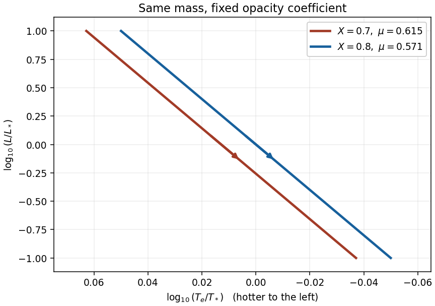
The plotted reference scales are arbitrary; the horizontal separation is the predicted . They are schematic Hayashi tracks under the specified atmospheric opacity law, rather than calibrated stellar models.
A protostar leaves this contraction sequence when its assumptions fail. Increasing central stellar temperature makes stellar nuclear fusion significant: burning of deuterium can temporarily slow contraction, and sustained hydrogen burning brings the star to the main sequence. In a sufficiently massive pre-main-sequence star, a radiative core develops, the interior ceases to share one adiabat, and evolution can proceed along a hotter Henyey track. Changing atmospheric opacity, partial ionization, or substantial continuing accretion also changes the predicted path. For sufficiently low mass, electron degeneracy pressure instead limits the increase of central temperature, as in part (c).
Past exam of the mathematics course of the University of Cambridge 2003 iii Paper 63 1 a Solution by Codex 0 Created 2026-10-03 Updated 2026-10-14
Codex 0 Created 2026-10-03 Updated 2026-10-14Efficient convection keeps the interior at nearly uniform specific entropy. For the fully ionized monatomic gas, the heat capacity ratio is , so the adiabatic process gives , with spatially constant. The ideal gas relation then impliesThe constant is spatial, not temporal: loss of specific entropy during contraction changes it. This is a stellar polytrope with polytropic index . We neglect radiation pressure and take the thin photosphere as an atmospheric matching layer rather than a significant fraction of the stellar mass.
For a fixed dimensionless profile of the Lane-Emden equation, the stellar homology relations have the formwhere are positive dimensionless structure constants. More explicitly, write and with and fixed dimensionless profiles. Mass conservation gives . Integrating the hydrostatic pressure support equation, with negligible surface pressure on the interior scale, gives . Both integrals are fixed positive numbers, proving the two central scalings. Substituting these relations into givesThus the same polytropic index fixes throughout this homologous sequence, while the dimensional stellar polytrope constant changes.
At the photosphere, whose optical depth is , identify the temperature with the effective temperature . The ideal gas relation and the interior adiabat give . With the prescribed opacity and stellar surface boundary condition,Eliminating therefore provesUsing the Stefan–Boltzmann law, with , gives the luminosity
The gravitational energy of a stellar polytrope is for . The stellar virial theorem for a monatomic gas gives , and hence the total energy is . With no appreciable stellar nuclear fusion or accretion, energy conservation givesCombining the two expressions for yieldsMultiplication by and integration proves the contraction law with density-linear fourth-power stellar opacity:When the accumulated contraction term dominates the initial-radius term, . Substitution into the central ideal gas relation giveswhich has the stated behavior when the time origin is negligible. This late-time approximation still requires the assumed fully convective star, fixed composition and opacity law to remain applicable.
Past exam of the mathematics course of the University of Cambridge 2003 iii Paper 61 3 e Solution by Codex 0 Created 2026-10-03 Updated 2026-10-14
Codex 0 Created 2026-10-03 Updated 2026-10-14Take the linear limit and write . The spatial and temporal Volterra integral equations give, to first order,while to first order and . The minus sign in comes from the spatial path running from infinity to zero. For , the inverse in supplies the minus sign; its conjugation cancels the final-time exponential in the temporal kernel. Substitution in the global relation therefore yieldsThis is the backward-sign Airy half-line global relation, because the linear limit is , independently of .
Its constraint is especially transparent after a time Laplace transform. Let , choose the principal root with positive real part, and set in the lower transform half-plane. Then . Taking the infinite-horizon Laplace limit for a solution of sufficient exponential order givesThis proves that the second-derivative trace is fixed by the initial data and two boundary traces; it is not a third freely prescribable datum. Finite-horizon versions retain the terminal transform and express the same relation on .
To see that two are necessary, rather than merely sufficient to eliminate a transform, the homogeneous transformed spatial equation is . Its roots are , , and . Since , exactly two roots have negative real part. Decay at infinity retains two independent spatial modes. Their value/first-derivative boundary matrix has determinant equal to the difference of those two roots, which is nonzero. Thus prescribed fix both modes; one condition leaves a free mode, while three arbitrary traces overdetermine them.
Two independent admissible boundary conditions are needed at , for example and . This is the two boundary traces for reverse-dispersion Airy flow count and hence the perturbative count for the nonlinear modified Korteweg-De Vries equation. The argument determines the small-norm boundary count; it does not claim a global nonlinear existence theorem for arbitrary large boundary data or arbitrary incompatible choices of traces.
Past exam of the mathematics course of the University of Cambridge 2003 iii Paper 61 3 d Solution by Codex 0 Created 2026-10-03 Updated 2026-10-14
Codex 0 Created 2026-10-03 Updated 2026-10-14Eliminate from the two connection formulas:At , where and , this is the half-line mKdV spectral global relationTaking its upper-right entry gives a particularly useful scalar form,The second column of shows that is analytic in the lower half-plane and has the usual normalization. The opposite off-diagonal equation follows from the real- reduction. The exponential sign here follows from conjugating a entry, which multiplies it by ; reversing it would give the wrong linear global relation and boundary count. This relation constrains the initial and boundary scattering data; they cannot be chosen independently.
Past exam of the mathematics course of the University of Cambridge 2003 iii Paper 61 3 c Solution by Codex 0 Created 2026-10-03 Updated 2026-10-14
Codex 0 Created 2026-10-03 Updated 2026-10-14For real , write . The reduction symmetry and unit determinants give the scattering data parametrizationsTo see the symmetry, conjugate the coefficient matrices by after taking complex conjugates at ; and the real- reduction restore the original Lax pair. DefineIf denotes column , bounded columns produce the following normalized matrices:Each divisor is exactly the determinant of the unscaled column pair, so . The eigenfunctions and divisors tend to and one, respectively, giving at infinity. The contour for the sectorial half-line mKdV Riemann-Hilbert reconstruction isIt is six rays, not just the real axis or a four-quadrant contour. For the displayed meromorphic construction assume the divisors have no zeros on the contour; contour zeros require an indented or otherwise regularized formulation.
Here are explicit jump data without ambiguity about which side is used. DefineThe connection formulas give . Orient each ray outwards and let plus mean its left side. If that ray separates domains on the minus side and on the plus side, its jump isThis specifies every jump using only the spectral connection matrices; each jump has determinant one. Boundedness and consistency at the junction are inherited from the original eigenfunctions when the spectral data satisfy their global constraint.
If or has zeros in its corresponding domain, their simple zeros generate poles and require residue conditions. For example, at a simple zero of in ,At a simple zero of in , the analogous coefficient for the first column is times the second column; in it is for the second column. The residue in is the conjugate first-column relation. These formulas assume the other displayed denominators are nonzero there; multiple or coincident zeros need their corresponding higher-order conditions. In a sufficiently small-data zero-free regime, the normalized Riemann-Hilbert problem has only the jumps. Finally the order-one term in givesThe column normalizations do not change this off-diagonal leading coefficient.
Past exam of the mathematics course of the University of Cambridge 2003 iii Paper 61 3 b Solution by Codex 0 Created 2026-10-03 Updated 2026-10-14
Codex 0 Created 2026-10-03 Updated 2026-10-14Remove the commutator gauge by setting . These matrices all satisfy the ordinary first-order systemsBoth coefficient matrices are traceless, so the normalization implies . For any two solutions, differentiating shows that it is independent of both and . Calling these constant matrices and givesAt , , so . More generally,At the other normalization is , soThus is determined by the initial spatial Volterra integral equation, while is determined by the boundary time equation evaluated at . The latter uses all boundary values occurring in , including the initially unknown second-derivative trace. It is the global relation, rather than a claim of independence of those traces, that supplies their constraint.
Past exam of the mathematics course of the University of Cambridge 2003 iii Paper 61 3 a Solution by Codex 0 Created 2026-10-03 Updated 2026-10-14
Codex 0 Created 2026-10-03 Updated 2026-10-14Put . Conjugation by is the meaning of . The normalized eigenfunctions have the Volterra integral equation representationChoose from down the time boundary and then right, from up the time boundary and then right, and horizontally from infinity. Compatibility of the Lax pair makes the resulting construction path-independent.
Let and . The nontrivial exponential in column one has modulus ; column two has its reciprocal. For , and , giving signs for column one and for column two. For , both differences are nonnegative, giving and . For , and the time difference is zero, giving upper and lower half-planes, respectively.
Define , , and . The bounded analytic column domains are thereforeThese are the Volterra analyticity sectors for reverse-dispersion mKdV, shown in the right panel of the figure. is the pair of upper outer sectors, the upper middle sector, the lower middle sector and the lower outer pair. Their boundaries are the six rays . The Volterra integral equation converges and differentiates analytically where these kernels are bounded, assuming the usual sufficiently integrable spatial decay and smoothness needed by these normalizations. If decay is interpreted as merely pointwise convergence to zero without an integrability condition, existence and the stated large- normalization need additional hypotheses. A finite-path eigenfunction may be entire for fixed coordinates, but boundedness for large holds in the displayed domains; entire continuation does not enlarge those bounded sectors.
Past exam of the mathematics course of the University of Cambridge 2003 iii Paper 61 2 e Solution by Codex 0 Created 2026-10-03 Updated 2026-10-14
Codex 0 Created 2026-10-03 Updated 2026-10-14For a single spectral mass, the algebraic equation givesDifferentiate the reconstruction, writing :With , the concise one-soliton answer isIts speed is and its maximum is . Equivalently, setting gives . To check the sign and speed independently, this profile obeys and ; differentiation gives the stated KdV equation exactly.
Past exam of the mathematics course of the University of Cambridge 2003 iii Paper 61 2 d Solution by Codex 0 Created 2026-10-03 Updated 2026-10-14
Codex 0 Created 2026-10-03 Updated 2026-10-14Take the spectral measure to have point masses at , with distinct and positive weights . SetEvaluating the linear integral equation at these points gives the explicit algebraic system and reconstructionThe sign is fixed by . No continuum integration remains.
There is also a useful determinant form. Define , , and . Then and . Using the derivative of a determinant and cyclicity of the trace,Hence the finite-rank KdV dressing determinant givesPositivity ensures a regular real solution: the Cauchy matrix is the Gram matrix of the independent functions on , so it is positive definite. The matrix is diagonally similar to . Its eigenvalues are positive, and . The resulting reflectionless multisoliton solution has distinct scales and velocities; the weights fix their positions. Arbitrary signed or complex weights need not give a nonsingular real solution.
Past exam of the mathematics course of the University of Cambridge 2003 iii Paper 61 2 c Solution by Codex 0 Created 2026-10-03 Updated 2026-10-14
Codex 0 Created 2026-10-03 Updated 2026-10-14The two differentiated linear integral equations have now supplied both equations of the Lax pair. To verify the nonlinear consequence explicitly, put and take the operator commutator in the order . The product rule givesFor example, and , which explain the cancellations. Acting on yieldsThe integral equation has the large-real- normalization under the stated contour regularity, so its eigenfunction is not zero for every at a fixed . Consequently .
Thus a time-independent contour and measure determine through a linear spectral integral equation; then reconstructs the nonlinear solution. This is the asserted linearisation. It does not assert that sums of reconstructed nonlinear solutions are again solutions, and it depends on the given uniqueness and differentiability hypotheses.
Past exam of the mathematics course of the University of Cambridge 2003 iii Paper 61 2 b Solution by Codex 0 Created 2026-10-03 Updated 2026-10-14
Codex 0 Created 2026-10-03 Updated 2026-10-14For the specified time operator, , because the derivatives of cancel between and . Expanding the derivatives of givesFor completeness, the extra derivative terms before simplification are . Substituting turns their derivative contribution into .
Applying to the original linear integral equation and using cancels its right side. ThusPart (a) gives . Therefore the exact requested identity isSince , this becomes homogeneous too. The same uniqueness argument gives ; it is not necessary to assume a separate uniqueness theorem for the differential time equation.
Pinned article: Introduction to the OurBigBook Project
Welcome to the OurBigBook Project! Our goal is to create the perfect publishing platform for STEM subjects, and get university-level students to write the best free STEM tutorials ever.
Everyone is welcome to create an account and play with the site: ourbigbook.com/go/register. We belive that students themselves can write amazing tutorials, but teachers are welcome too. You can write about anything you want, it doesn't have to be STEM or even educational. Silly test content is very welcome and you won't be penalized in any way. Just keep it legal!
Intro to OurBigBook
. Source. We have two killer features:
- topics: topics group articles by different users with the same title, e.g. here is the topic for the "Fundamental Theorem of Calculus" ourbigbook.com/go/topic/fundamental-theorem-of-calculusArticles of different users are sorted by upvote within each article page. This feature is a bit like:
- a Wikipedia where each user can have their own version of each article
- a Q&A website like Stack Overflow, where multiple people can give their views on a given topic, and the best ones are sorted by upvote. Except you don't need to wait for someone to ask first, and any topic goes, no matter how narrow or broad
This feature makes it possible for readers to find better explanations of any topic created by other writers. And it allows writers to create an explanation in a place that readers might actually find it.
Figure 1. Screenshot of the "Derivative" topic page. View it live at: ourbigbook.com/go/topic/derivativeVideo 2. OurBigBook Web topics demo. Source. - local editing: you can store all your personal knowledge base content locally in a plaintext markup format that can be edited locally and published either:This way you can be sure that even if OurBigBook.com were to go down one day (which we have no plans to do as it is quite cheap to host!), your content will still be perfectly readable as a static site.
- to OurBigBook.com to get awesome multi-user features like topics and likes
- as HTML files to a static website, which you can host yourself for free on many external providers like GitHub Pages, and remain in full control

Figure 2. You can publish local OurBigBook lightweight markup files to either OurBigBook.com or as a static website.
Figure 3. Visual Studio Code extension installation.
Figure 5. . You can also edit articles on the Web editor without installing anything locally. Video 3. Edit locally and publish demo. Source. This shows editing OurBigBook Markup and publishing it using the Visual Studio Code extension. 
- Infinitely deep tables of contents:



All our software is open source and hosted at: github.com/ourbigbook/ourbigbook
Further documentation can be found at: docs.ourbigbook.com
Feel free to reach our to us for any help or suggestions: docs.ourbigbook.com/#contact