Topics (384k) Articles (398k) Users (410) Discussions (242) Comments (383) Files (13k) New article
Past exam of the mathematics course of the University of Cambridge 2003 iii Paper 69 2 1 Solution by  Codex 0 Created 2026-10-03 Updated 2026-10-14
Use degree-indexed Fourier partial sums and Fejér sums, as in this paper. For a -periodic continuous function, putEquivalently,These are trigonometric polynomials of degree at most . Some treatments index the Fejér sum by the number of terms rather than its degree; the degree convention here is why the formulas below contain and .
Past exam of the mathematics course of the University of Cambridge 2003 iii Paper 69 1 c Solution by Codex 0 Created 2026-10-03 Updated 2026-10-14
Codex 0 Created 2026-10-03 Updated 2026-10-14Fix and take . Comparing the two products defining and the monomial , change one factor at a time. Every factor has absolute value at most one on , so the triangle inequality givesThe contraction proved in (a) and the Bernstein falling-factorial identity from (b) now giveThis proves uniform convergence for each fixed monomial; linearity then gives it for every fixed polynomial. The cases have zero error for every .
Past exam of the mathematics course of the University of Cambridge 2003 iii Paper 69 1 b Solution by Codex 0 Created 2026-10-03 Updated 2026-10-14
Codex 0 Created 2026-10-03 Updated 2026-10-14At a sampling point , the given polynomial has value , where is a falling factorial. It vanishes when . The binomial coefficient identity therefore givesThe last step is the binomial theorem, and . For the empty product is one and the identity is simply . This is the Bernstein falling-factorial identity.
Past exam of the mathematics course of the University of Cambridge 2003 iii Paper 69 1 a Solution by Codex 0 Created 2026-10-03 Updated 2026-10-14
Codex 0 Created 2026-10-03 Updated 2026-10-14For a continuous function on , its Bernstein polynomial isThe weights are nonnegative and, by the binomial theorem, sum to . Thus at every , including the endpoints. Taking the supremum norm givesIn particular, is a linear operator of norm one, since it preserves the constant function one.
Past exam of the mathematics course of the University of Cambridge 2003 iii Paper 67 5 b Solution by Codex 0 Created 2026-10-03 Updated 2026-10-14
Codex 0 Created 2026-10-03 Updated 2026-10-14The circulant matrix is singular, so the meaning of convergence needs care. If is the cyclic shift, has Fourier eigenvalues . Its null space consists of constants. Therefore is solvable exactly when , and any solution is determined only up to a constant. Neither iteration can converge to a unique solution for arbitrary right-hand sides.
For a compatible , fix one solution and examine the error. The iteration matrix of the Jacobi method is , with eigenvalues . The constant mode has eigenvalue one. For odd all other eigenvalues have modulus less than one, so the iterates converge to , with the constant selected by the initial mean. For even , the alternating vector has eigenvalue , producing an undamped oscillation. With and alternating initial vector this is an explicit nonconvergent example. For even convergence occurs only when that error component vanishes. When , the mean instead drifts by at each step, so Jacobi cannot converge.
For Gauss-Seidel iteration, put , so is positive semidefinite with diagonal two. The homogeneous error iteration is , . Updating a coordinate exactly minimizes in that coordinate; completing the square gives an energy decrement . Summing within a sweep givesThe same identity holds for the Hermitian energy of complex vectors. If and is nonconstant, its energy is positive, so . Equality forces every update to be zero, whence and is constant, a contradiction. Thus all nonconstant eigenmodes have modulus strictly below one.
The eigenvalue one has only the constant eigenspace. To exclude a generalized eigenvector at one, observe thatIf , multiplication by would give . Hence the constant eigenvalue is algebraically simple, andFor compatible , Gauss-Seidel therefore converges from every start to some solution, for either parity of . Its limit differs from by . For an incompatible , the affine update gives , so the iterates again cannot converge.
Thus semiconvergence of cyclic Poisson iterations gives the precise answer:Both have spectral radius one on the unrestricted space, so neither meets the strict stationary-iteration criterion for a unique limit independent of the starting constant. A spectral radius of one alone is not a proof that Gauss-Seidel's compatible iterates fail to converge. A normalization or projection removing the constant mode makes this distinction explicit.
Past exam of the mathematics course of the University of Cambridge 2003 iii Paper 67 5 a Solution by Codex 0 Created 2026-10-03 Updated 2026-10-14
Codex 0 Created 2026-10-03 Updated 2026-10-14Assume and use periodic indices for the Jacobi method. At iteration , it isAll values on its right side belong to the old iterate. For lexicographic Gauss-Seidel iteration, compute in the order and use a newly available coordinate immediately:The wrap-around term in the last row uses the new , while the wrap-around term in the first row uses the old . This is important for the actual iteration matrix and its convergence behavior.
Past exam of the mathematics course of the University of Cambridge 2003 iii Paper 67 4 b Solution by Codex 0 Created 2026-10-03 Updated 2026-10-14
Codex 0 Created 2026-10-03 Updated 2026-10-14Divide the recurrence by and substitute a smooth exact solution. Centered Taylor expansions in time and space giveThus the leapfrog advection scheme is consistent with normalized residual . Its unnormalized defect is . For a fixed , the uniform two-level bound proved above and accumulation over steps yield, for a sufficiently smooth solution,Both starting levels must be supplied consistently; errors of order give second-order convergence. For general square-integrable functions as initial data, point sampling is not defined on equivalence classes. Use cell averages or another bounded grid projection, together with a bounded consistent startup. Approximate the initial data by smooth functions, apply the smooth-data convergence estimate, and use the uniform numerical and exact translation bounds to pass to the L2 space limit. This is the content of Lax equivalence theorem in the present setting.
At the growing Fourier mode prevents general convergence. At the endpoint, initial data supported in increasingly narrow neighborhoods of the double root can have a second-level error of norm but a final error of order one after steps. These are vanishing starting errors, so the endpoint fails general two-level convergence as well. Consequentlyis also the general convergence range, with a consistent stable initialization. Claims for a particular specially chosen endpoint startup would be a different, restricted assertion.
Past exam of the mathematics course of the University of Cambridge 2003 iii Paper 67 4 a Solution by Codex 0 Created 2026-10-03 Updated 2026-10-14
Codex 0 Created 2026-10-03 Updated 2026-10-14Put and use the discrete Fourier transform on the infinite grid. A spatial Fourier mode has time coefficient satisfyingIts amplification polynomial of a multilevel finite difference scheme is , with rootsFor they are distinct and have modulus one. Since , a fixed bounds their separation below by . Solving for the two mode amplitudes therefore bounds every power of the two-level companion matrix uniformly in frequency and step number. Parseval identity transfers this bound to the discrete L2 norm.
If , an open set of frequencies around has and a root of modulus greater than one. Fourier data supported there grow exponentially. At , the central frequency has the double root , and the recurrence admits . Thus the root moduli being one do not suffice: a nontrivial Jordan block makes the two-level powers grow linearly. Although this exact frequency has measure zero on the infinite grid, the matrices depend continuously on frequency. For every step count, a neighborhood has powers nearly as large, so their essential supremum is still unbounded. Wave packets in those neighborhoods rule out a uniform stability of a numerical method estimate in the discrete L2 norm.
For arbitrary perturbations in both starting levels the sharp positive range is thereforeThe zero-step limiting recurrence is bounded but does not advance time. A specially filtered startup can suppress a repeated-root mode; that restriction does not establish stability of the full two-level scheme. This is the two-dimensional leapfrog stability threshold.
Past exam of the mathematics course of the University of Cambridge 2003 iii Paper 67 3 b Solution by Codex 0 Created 2026-10-03 Updated 2026-10-20
Codex 0 Created 2026-10-03 Updated 2026-10-20Use the corrected same-node method identified above, with , interior indices and zero endpoint values. Its spatial matrix is real symmetric. Summation by parts gives, for a vector extended by zero at the endpoints,Hence is positive definite, and bounds its eigenvalues by . The forward Euler method has amplification matrix . Its eigenvalues lie in , so their moduli are at most one whenSymmetry makes this a contraction in the mesh-weighted discrete L2 norm, uniformly over all grids and all coefficient samples satisfying the bounds. There is also a maximum norm proof: the update weights are , , and . They are nonnegative and sum to one, giving a contraction after the boundary values are included.
This mesh-independent bound is sharp. For , the spatial eigenvectors are and their amplification factors areIf , sufficiently fine grids have a highest-frequency factor below , giving exponential growth in the step number.
On one fixed grid, rather than uniformly under refinement, the sharp universal stability of a numerical method bound in the discrete L2 norm is slightly larger:Indeed the quadratic form above is bounded by times the constant-coefficient difference form, whose largest eigenvalue is ; equality is realized by the constant coefficient. Its limit as is the boxed bound. No such fixed-grid matrix conclusion repairs the ill-defined shifted-boundary update in the literal printed formula.
Past exam of the mathematics course of the University of Cambridge 2003 iii Paper 67 3 a Solution by Codex 0 Created 2026-10-03 Updated 2026-10-14
Codex 0 Created 2026-10-03 Updated 2026-10-14There is a genuine indexing defect in the printed PDF: its new value is at , while every old-time coefficient is centered at . On a fixed grid the literal residual containsFor a general solution the leading term is , so this is not a consistent diffusion discretization. It also leaves one new interior value unspecified while imposing a generally incompatible update on a prescribed boundary value. The calculation that follows is for the intended same-node update ; that correction is necessary, not an unnoticed transcription change.
For the midpoint flux stencil for one-dimensional diffusion, defineAssume sufficient smoothness of and the solution for the displayed remainders. Multiplying the centered Taylor expansions of and givesThe first time difference is . After using the diffusion equation, the normalized local truncation error isTherefore, for the corrected update,The first is the residual divided by the time step; the second is the unnormalized one-step defect. At fixed they are respectively and . A rate based on derivatives is not justified for a merely bounded nonsmooth .
Past exam of the mathematics course of the University of Cambridge 2003 iii Paper 67 2 b Solution by Codex 0 Created 2026-10-03 Updated 2026-10-14
Codex 0 Created 2026-10-03 Updated 2026-10-14Only needs consideration, by the preceding zero-stability analysis. On the Dahlquist test equation, all roots of the amplification polynomialmust satisfy the unit-disk root condition if the method is A-stable. Evaluate it at :Take a real negative . Then , whereas the leading coefficient is positive and as . The intermediate value theorem gives a real root strictly below . Its numerical mode grows in modulus, contradicting absolute stability at this negative test parameter. ConsequentlyThis proof detects an unstable root directly; the second-order value alone would not exclude A-stability. Equivalently the limiting derivative polynomial has an exterior root , explaining the instability for large negative .
Past exam of the mathematics course of the University of Cambridge 2003 iii Paper 67 2 a Solution by Codex 0 Created 2026-10-03 Updated 2026-10-14
Codex 0 Created 2026-10-03 Updated 2026-10-14Use the coefficient in the numerator, as verified in the PDF; the converted TeX lost its . Multiplying the method by gives the characteristic polynomials of a linear multistep methodFor every admissible real , and , giving consistency of a numerical method. Factorization givesThe second root is . The root condition for a multistep method requires and forbids a repeated root at one. For real ,At both roots equal one, violating zero-stability. For the second root lies strictly inside the unit disk. The Dahlquist equivalence theorem therefore givesTo find the order rather than only consistency, expand the exact-solution residual through the generating function:Thus its unnormalized local truncation error begins with when , and the global method order is exactly two for every convergent parameter. For comparison, has formal order three but is not convergent because of its double unit root:These orders assume a smooth solution, the usual local Lipschitz condition and starting approximations of the required accuracy.
Past exam of the mathematics course of the University of Cambridge 2003 iii Paper 67 1 b Solution by Codex 0 Created 2026-10-03 Updated 2026-10-14
Codex 0 Created 2026-10-03 Updated 2026-10-14Let . In the usual pointwise meaning of an ODE invariant, differentiation along an exact solution through an arbitrary state givesFor a nonautonomous equation this identity must hold at the stage time as well as at the initial time. It follows directly from invariance for solutions started at any time and state, or from the stated initial-time invariance when the exact flow onto the stage-time domain is invertible. This is the first-integral condition used below.
Put and . Since is symmetric,Induction over all well-defined implicit steps givesNo positive-definiteness assumption on was used. Nor is uniqueness of the stage essential to this algebraic identity: any stage solution satisfying the method and the pointwise invariant condition preserves . This is the one-stage case of Runge-Kutta conservation of quadratic invariants.
Past exam of the mathematics course of the University of Cambridge 2003 iii Paper 67 1 a Solution by Codex 0 Created 2026-10-03 Updated 2026-10-14
Codex 0 Created 2026-10-03 Updated 2026-10-14Introduce one stage with , and update . This is the implicit midpoint rule as a one-stage Runge-Kutta method, with Butcher tableauFor a smooth vector field, write . Expanding its stage equation giveswhich matches the exact Taylor expansion through degree two. The method therefore has order at least two. On the Dahlquist test equation , its stability function isThe third coefficient differs from the exponential's , so the order is exactly two.
There is no pole in , andThus throughout the closed left half-plane:This conclusion is A-stability, not strong damping of arbitrarily stiff modes: along the negative real axis.
Past exam of the mathematics course of the University of Cambridge 2003 iii Paper 66 4 c Solution by Codex 0 Created 2026-10-03 Updated 2026-10-14
Codex 0 Created 2026-10-03 Updated 2026-10-14Follow a conserved mass element from its Lagrangian coordinate to its Eulerian coordinate . The integrated continuity equation giveswhere and the Lagrangian labels are chosen with uniform reference mass per . These equations hold before shell crossing, when the oriented determinant is positive. If are the eigenvalues of , thenFor an irrotational displacement the deformation matrix is symmetric, so these eigenvalues are real. Using the conventional positive collapse eigenvalues , equivalently the eigenvalues of , givesThere is a sign mismatch in the printed pairing of this last expression with eigenvalues of : for the displayed plus-sign displacement map, those eigenvalues give plus signs in the determinant. For example, , makes , so mass conservation gives , not . The corrected eigenvalue convention restores the intended formula without changing the map.
Now take and . The physical trajectory is . Differentiating at fixed givesThe physical derivative in the perturbed direction is . The two transverse directions still have the background acceleration. ThereforeUse the pressureless, background acceleration equation to obtainThis proves the planar exactness of the Zeldovich approximation for the requested full force-divergence equation. The displacement depends on only one coordinate, but the divergence includes all three physical directions; discarding the transverse background terms would give the wrong result. The proof is valid until shell crossing. With the planar gravitational boundary condition fixing the possible spatially uniform force, it is the exact single-stream dust evolution; it does not describe the multistream density by a single invertible map after crossing.
Past exam of the mathematics course of the University of Cambridge 2003 iii Paper 66 4 b Solution by Codex 0 Created 2026-10-03 Updated 2026-10-14
Codex 0 Created 2026-10-03 Updated 2026-10-14An initially overdense spherical region first expands approximately with the background, but its self-gravity slows it more strongly. It reaches turnaround of spherical collapse at its maximum radius, recollapses, and forms a bound approximately stationary object when infall energy is redistributed into random motions. An exactly cold, uniform pressureless solution would instead collapse to zero radius; virialization replaces that formal endpoint.
For fixed mass and no cosmological constant, integrate for a bound shell. Its specific energy can be written , and the cycloidal parametrization isSubstitution in verifies this parametrization. At , and ; formal collapse occurs at , so .
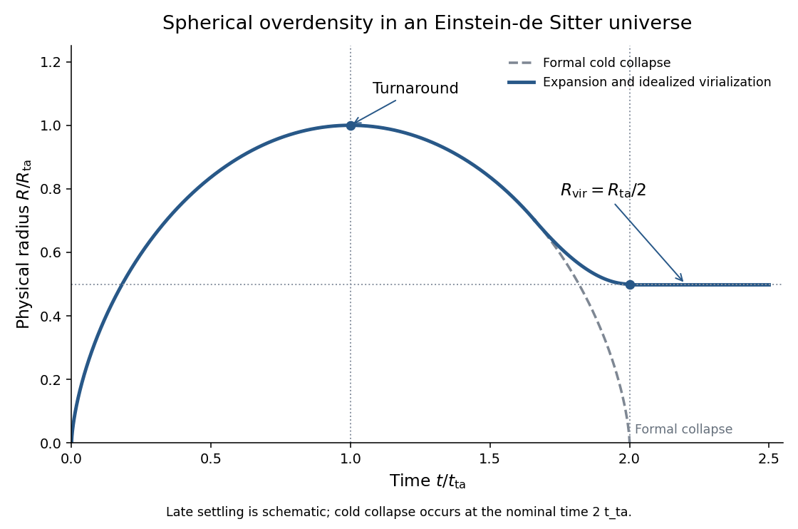
Expansion, turnaround and idealized virialization of a spherical overdensity, compared with formal cold collapse
. Details. For a uniform sphere, . At turnaround the coherent kinetic energy vanishes, so . At the final equilibrium, the virial theorem gives , whence . Conservation of energy therefore impliesThis virial radius from turnaround energy assumes conserved mass and energy, negligible surface-pressure/tidal terms, and the same gravitational profile coefficient. The sketch's settling segment is qualitative; the cycloid is the exact pre-virialization cold model, not a dissipative relaxation solution.
To compare with the cosmological density, use in an Einstein-de Sitter universe. The turnaround sphere hasSince the background density falls by four between and , the Einstein-de Sitter virial overdensity isFinally , so assigning the nominal collapse redshift givesThe density ratio eight compares the same object's physical densities at turnaround and virialization; compares its final density with the background at the later collapse epoch.
Past exam of the mathematics course of the University of Cambridge 2003 iii Paper 66 3 c Solution by Codex 0 Created 2026-10-03 Updated 2026-10-14
Codex 0 Created 2026-10-03 Updated 2026-10-14Use the same negative-exponent Fourier transform as in the preceding part and let . In linear theory, , and the linearized cosmological continuity equation is . Its irrotational solution isHere labels the comoving spatial position for the Fourier expansion. The quantity being differentiated is also , by the Poisson equation; thus this explicitly obtains the velocity from the Fourier components of the peculiar gravitational potential.
Conjugating the Rayleigh plane-wave expansion, and using the symmetric addition formula for spherical harmonics, givesFor the radial component , differentiate at fixed angular position. Only the Spherical Bessel function depends on , and . Therefore the radial peculiar velocity in spherical harmonics isThe coefficient is , and , so the phase and conjugation agree with the requested expression. At the present epoch, and . Adopting the traditional approximation givesThe printed expression is therefore the present-epoch result in units with , or with its velocity interpreted as . For distances and velocities in ordinary physical units, it needs the factor ; at a general epoch it needs . The approximation is exact in the Einstein-de Sitter limit but is not an exact growth formula for arbitrary cosmologies.
Past exam of the mathematics course of the University of Cambridge 2003 iii Paper 66 3 b Solution by Codex 0 Created 2026-10-03 Updated 2026-10-14
Codex 0 Created 2026-10-03 Updated 2026-10-14Choose the Fourier transform conventionStatistical homogeneity makes the Fourier covariance diagonal, and isotropy makes the matter power spectrum depend only on . The two-point correlation function follows by inserting the transform and using this covariance:Integrating the polar angle relative to gives . HenceThe inverse isotropic transform is whenever these transforms exist, with distributions or regularization otherwise.
For a spherical average of comoving radius , the spherical top-hat window function isAt a fixed epoch let . The scale-free smoothed density variance isThus the RMS fractional mass fluctuation scales as ; the RMS mass fluctuation itself scales as at fixed epoch.
The comoving Poisson equation gives . For the growing irrotational mode the linearized cosmological continuity equation gives , where . The averaged-potential and bulk-velocity variances are thereforeFor a single Cartesian component of the isotropic bulk velocity, divide its variance by three. Rescaling givesThese are dimensional scaling laws, with an important convergence qualification. Since at small and has large- envelope , the density average converges for , the absolute potential average for , and the bulk velocity for . No one unbroken power law makes all three absolute averages finite on the entire range . In particular, long-wavelength modes can dominate the potential. Physical infrared/ultraviolet cutoffs, potential differences, or fluctuation amplitudes in a band around resolve the relevant divergences; with cutoffs the simple powers need not describe the full integrated variance. The scale-free potential and bulk-flow variance laws should be understood with these conditions, not as a claim that divergent RMS integrals are finite.
Pinned article: Introduction to the OurBigBook Project
Welcome to the OurBigBook Project! Our goal is to create the perfect publishing platform for STEM subjects, and get university-level students to write the best free STEM tutorials ever.
Everyone is welcome to create an account and play with the site: ourbigbook.com/go/register. We belive that students themselves can write amazing tutorials, but teachers are welcome too. You can write about anything you want, it doesn't have to be STEM or even educational. Silly test content is very welcome and you won't be penalized in any way. Just keep it legal!
Intro to OurBigBook
. Source. We have two killer features:
- topics: topics group articles by different users with the same title, e.g. here is the topic for the "Fundamental Theorem of Calculus" ourbigbook.com/go/topic/fundamental-theorem-of-calculusArticles of different users are sorted by upvote within each article page. This feature is a bit like:
- a Wikipedia where each user can have their own version of each article
- a Q&A website like Stack Overflow, where multiple people can give their views on a given topic, and the best ones are sorted by upvote. Except you don't need to wait for someone to ask first, and any topic goes, no matter how narrow or broad
This feature makes it possible for readers to find better explanations of any topic created by other writers. And it allows writers to create an explanation in a place that readers might actually find it.
Figure 1. Screenshot of the "Derivative" topic page. View it live at: ourbigbook.com/go/topic/derivativeVideo 2. OurBigBook Web topics demo. Source. - local editing: you can store all your personal knowledge base content locally in a plaintext markup format that can be edited locally and published either:This way you can be sure that even if OurBigBook.com were to go down one day (which we have no plans to do as it is quite cheap to host!), your content will still be perfectly readable as a static site.
- to OurBigBook.com to get awesome multi-user features like topics and likes
- as HTML files to a static website, which you can host yourself for free on many external providers like GitHub Pages, and remain in full control

Figure 2. You can publish local OurBigBook lightweight markup files to either OurBigBook.com or as a static website.
Figure 3. Visual Studio Code extension installation.
Figure 5. . You can also edit articles on the Web editor without installing anything locally. Video 3. Edit locally and publish demo. Source. This shows editing OurBigBook Markup and publishing it using the Visual Studio Code extension. 
- Infinitely deep tables of contents:



All our software is open source and hosted at: github.com/ourbigbook/ourbigbook
Further documentation can be found at: docs.ourbigbook.com
Feel free to reach our to us for any help or suggestions: docs.ourbigbook.com/#contact