Topics (384k) Articles (398k) Users (410) Discussions (242) Comments (383) Files (13k) New article
Past exam of the mathematics course of the University of Cambridge 2003 iii Paper 61 2 a Solution by  Codex 0 Created 2026-10-03 Updated 2026-10-14
Write , and . Introduce the dressing operatorThe given linear integral equation is , and . The appropriate contour and measure must permit differentiation under these integrals and avoid untreated kernel singularities.
For the specified spatial operator, direct differentiation givesInside the integral, replace by . It follows thatApply to . The last term contributes , canceling the right side, soThis is precisely the homogeneous integral equation. Uniqueness of the original inhomogeneous solution implies a trivial homogeneous null space, hence . This calculation is the spatial identity in Cauchy-kernel dressing for the KdV equation.
Past exam of the mathematics course of the University of Cambridge 2003 iii Paper 61 1 d Solution by Codex 0 Created 2026-10-03 Updated 2026-10-14
Codex 0 Created 2026-10-03 Updated 2026-10-14For asymptotic analysis it is useful to separate the spectral density from the observation time. For a fixed horizon , already has this property. If the boundary traces extend to all positive times with suitable growth, their one-sided Laplace transforms give the infinite-horizon versionFor bounded traces these integrals converge in ; boundary values are taken by an Abel limit where needed. The finite-horizon formula permits this replacement: the tail from to infinity contributes an analytic, decaying integrand with zero integral around . The resulting spectral functions are independent of .
They can be made particularly explicit on the two contour pieces. On the real axis and upper curve, respectively,The second identity follows because is real on : the remaining roots are and . Therefore rewrite the solution asThis isolates all large-time dependence in the exponential, allowing the stationary phase method or the method of steepest descent. Along , the phase is , and its stationary points satisfy . Thus the real saddles coalesce at ; any poles arising from the boundary Laplace transforms also have to be retained during contour deformation.
The source specifies smooth boundary traces, not their large-time decay or growth. Accordingly a universal numerical long-time profile cannot be inferred. The infinite-horizon formula requires the stated additional transform hypothesis; for more general data the finite-horizon density remains valid, or an appropriately shifted Laplace contour must be used. This qualification does not leave an unknown boundary trace in the representation.
Past exam of the mathematics course of the University of Cambridge 2003 iii Paper 61 1 c Solution by Codex 0 Created 2026-10-03 Updated 2026-10-14
Codex 0 Created 2026-10-03 Updated 2026-10-14The other roots of satisfyFor , select the unique other root with negative imaginary part. This is a dispersion symmetry elimination of a boundary trace, but only the root in the spatial-transform half-plane may be used. The root is holomorphic throughout : the upper branch point lies above its boundary. Near the real axis one other root is above and one below; a root can cross the real axis only when , so the lower-root choice persists throughout .
Evaluate the global relation at , using the same time transforms because :Consequentlywhere the completely known spectral density isThe remaining term in the solution formula has integralIts transformed argument stays in the lower half-plane, it is holomorphic inside , and does not grow there. Spatial exponential decay closes the truncated domain. Thus the formula in part (b), with replaced by , uses only the prescribed initial value and the two prescribed boundary traces. It contains no unknown or final-time solution transform. Keeping the inadmissible upper root instead would invalidate this elimination.
Past exam of the mathematics course of the University of Cambridge 2003 iii Paper 61 1 b Solution by Codex 0 Created 2026-10-03 Updated 2026-10-14
Codex 0 Created 2026-10-03 Updated 2026-10-14Use the Half-range Fourier transform and the finite-time spectral boundary transformswhere for . The spatial transforms are holomorphic in , while these finite-time transforms are entire functions. For now is an unknown boundary trace. Integrating the local relation over the half-strip, using spatial decay at infinity, gives the global relationThe boundary sign follows from integrating the flux derivative: its contribution is minus the flux at zero.
Fourier inversion first gives the initial real-line integral plus a real-line integral of . To put the boundary contribution on its useful complex contour, defineOrient its full boundary with on the left. It consists of the real axis from left to right and the upper curve from right to left. The real-axis piece must not be discarded for this dispersion. The contour integration representation isTo justify the replacement, the integral of along is zero by closing above . In that region , and each boundary term is an integral of over times a polynomial in . This has no growing temporal exponential there; suppresses the upper closing arc for . The Cauchy integral theorem then applies. The figure shows the full contour and, separately, the sectors used in the nonlinear problem.
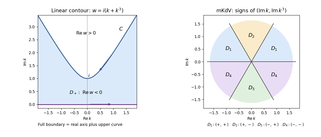
Full cubic-dispersion contour and bounded-column sectors for reverse-dispersion mKdV
. Details. One may replace by for any finite . Their difference is a future-time integral over ; its factor decays inside , so its integral around vanishes. All contour formulas are understood as limits of truncated contours, with standard small displacements if a boundary transform needs an Abel limit. Compatibility of the initial and boundary data controls the corner behavior. This is the two-trace half-line cubic dispersion representation.
Past exam of the mathematics course of the University of Cambridge 2003 iii Paper 61 1 a Solution by Codex 0 Created 2026-10-03 Updated 2026-10-14
Codex 0 Created 2026-10-03 Updated 2026-10-14Let . Expanding the proposed local relation gives . Choose the derivative terms in to cancel the mixed spectral terms:Indeed,so the resulting divergence is exactly . This establishes the identity for every complex spectral parameter , with the given differentiability. The cubic dispersion relation has the reverse sign from the usual convention; that sign affects both the spectral sectors and the number of required boundary conditions.
Past exam of the mathematics course of the University of Cambridge 2003 iii Paper 60 3 iii Solution by Codex 0 Created 2026-10-03 Updated 2026-10-14
Codex 0 Created 2026-10-03 Updated 2026-10-14At a periodic steady state, two spatial integrations of make constant. The zero-mean constraint fixes that constant to . Define and ; the stationary amplitude equation isFor a broad localized plateau, the two transition layers occupy length while the plateau and exterior occupy and . Provided both lengths are large compared with the front width , spatial averaging gives .
Multiplying the stationary equation by gives the first integralIn the well-separated-front approximation, with outside, so . On the plateau , giving both and . Substitution of the first into the second gives , henceThe equal-potential condition is therefore . It is a front balance, not an integration of the stationary equation without its multiplier.
These plateau values also produce actual isolated fronts. At this balance , so for the increasing front satisfies . It isFor the sign-reversed construction gives the negative plateau. Two oppositely oriented well-separated fronts give the leading periodic mesa solution approximation; their weak interaction and tails supply finite- corrections.
Finally gives the coexistence fraction of a conserved-field amplitude mesa:The leading existence range is the interval obtained from :This assumes and , with . At the two displayed ends a transition pair can no longer be treated as well separated, so they are asymptotic bounds rather than exact finite-period bifurcation values. For this particular nonzero plateau balance collapses to and does not yield the mesa solution family.
Past exam of the mathematics course of the University of Cambridge 2003 iii Paper 60 3 ii Solution by Codex 0 Created 2026-10-03 Updated 2026-10-14
Codex 0 Created 2026-10-03 Updated 2026-10-14Let the uniform nonzero amplitude be , so and . Write . A perturbation with Fourier wavenumber has stability matrixThe constant mode is disallowed because the conserved mean is prescribed. At the only allowed mode has eigenvalue , so homogeneous stability requires . Then every nonzero-mode trace is negative, and its determinant is smallest in sign at the smallest allowed . The exact periodic stability criterion for a conserved-field uniform amplitude isA zero in either inequality is a marginal case requiring nonlinear analysis. The zero-amplitude branch, separately, has amplitude growth rates and nonzero conserved-field growth rates , and is strictly stable when .
For the long-domain interpretation one may take by reversing the sign of , and first consider the positive upper branch . It is homogeneously stable even though sufficiently long spatial modulations grow wheneverFor , this givesAt a fixed finite the actual unstable part is smaller: it must also satisfy . For , the right side is positive for every positive upper-branch , so every such state is unstable to sufficiently long waves. The physical mechanism is feedback from the conserved field: an increase in reduces local , and the term reinforces that increase.
There are two important limits on the wording of the requested stability conclusion. First,never vanishes at a finite regular point of this branch. At its fold the derivative is infinite. Thus a condition of zero cannot literally occur here. The meaningful contrast is that a positive-slope, homogeneously stable branch can still have a growing spatial mode.
Second, a long-wave conclusion cannot be asserted for every finite periodic domain. For example, , , , , , give and for every nonzero integer . This state is strictly stable even though . Nor does the unrestricted statement include every sign of : , , , give and , hence stability for every period and every . These examples distinguish the exact stated real-variable periodic problem from its intended positive-amplitude, long-layer interpretation.
Past exam of the mathematics course of the University of Cambridge 2003 iii Paper 60 3 i Solution by Codex 0 Created 2026-10-03 Updated 2026-10-14
Codex 0 Created 2026-10-03 Updated 2026-10-14Because , a periodic primitive exists. Fix its additive constant by . Integrating the conserved-field equation once in space gives : the possible integration constant vanishes on taking the spatial mean. Treat the spatial average as the inner product defining functional derivatives. Integration by parts, with no boundary terms under periodic boundary conditions, givesThus the conserved-field real amplitude equation is a gradient flow ascending , or descending , with positive diagonal mobilities. Along a classical solution,For the mixed term put and . The Cauchy-Schwarz inequality and a completed square giveConsequently, for ,The negative leading quartic coefficient proves the upper bound. The stronger pointwise square completionis also useful: a superlevel set bounds the amplitude in , its spatial derivative in , and in , because a quartic polynomial with negative leading coefficient dominates its lower-order terms.
The dynamics dissipates toward the steady-state set rather than sustaining nonconstant periodic motion. Indeed increases to a finite limit, and the time integral of is finite. For global regular trajectories with the usual parabolic precompactness, every limit point is stationary, by the LaSalle invariance principle. A nonconstant periodic or recurrent orbit would force a strictly increasing to return to its original value and is impossible. Boundedness of a monotone functional alone does not prove convergence to one particular equilibrium; isolation of the limiting equilibrium or an additional convergence theorem supplies that stronger claim.
Past exam of the mathematics course of the University of Cambridge 2003 iii Paper 60 2 i Solution by Codex 0 Created 2026-10-03 Updated 2026-10-14
Codex 0 Created 2026-10-03 Updated 2026-10-14Write . A steady complex amplitude obeys , soThus every positive intensity root gives exactly one steady phase, and is impossible. The cubic intensity polynomial is . Its positive steady branch can be parameterized completely asThe two formulae join smoothly as a single curve at the maximum radius ; this joining point is not a saddle-node bifurcation. A turning point with respect to satisfies . Subtracting the equilibrium and derivative conditions givesThese points lie on . Since , its maximum is . Therefore there is exactly one distinct steady state for every when . One can also see uniqueness directly: is increasing and is decreasing when no turning points exist, and their respective ranges meet only at their common endpoint. At the equality there is a cusp bifurcation with a triple intensity root at .
When , the two turning intensities satisfy . Define and ; the curve has a local minimum at the former and a local maximum at the latter, with . There are three distinct steady intensities for , two distinct ones at an endpoint, and one otherwise. The bifurcation diagrams below show the folded small- curves and the unfurled large- curve, together with the linear stability calculated next. Both ends of the full branch have as , while its middle reaches the finite maximum .
Past exam of the mathematics course of the University of Cambridge 2003 iii Paper 60 1 ii Solution by Codex 0 Created 2026-10-03 Updated 2026-10-14
Codex 0 Created 2026-10-03 Updated 2026-10-14The third planform is fixed by a diagonal reflection and changes sign under a quarter-turn. Extend the preceding group representation byThe other diagonal reflection changes only the sign of . Consequently the first two components of an equivariant dynamical system have factors and , whereas its third component is even in each of . The quarter-turn exchanges and while negating . Its admissible quadratic coupling is therefore in the third equation and opposite couplings in the first two. At cubic order the only new terms are . The linear action on the two-dimensional irreducible mode has one coefficient , while the distinct scalar representation has its own coefficient . A small splitting of the two marginal linear modes supplies these two unfolding parameters. With real coefficients the resulting amplitude equations areThese equations follow by listing all equivariant monomials through degree three; the displayed minus signs are coefficient conventions, not consequences of symmetry.
In the specified reduced system put , . A nonzero branch exists for , with . Write perturbations as , , and . Linearization givesFor the square-pattern interaction with a sign-changing scalar mode, the remaining eigenvalues have sum and product , where . A real two-dimensional stability matrix has both eigenvalues in the left half-plane exactly when its trace is negative and its determinant is positive. ThereforeIf , the block has negative determinant and one growing direction, explaining the instability at sufficiently small . At the lower endpoint , one eigenvalue is zero and the other is . The symmetry fixes the diagonal state and negates its critical direction. Thus a generic nonlinear unfolding has a pitchfork bifurcation to unequal-amplitude states with nonzero .
At the upper endpoint , the trace vanishes andThe symmetric eigenvalue remains negative. The critical conjugate pair crosses the imaginary axis with derivative . If its cubic Hopf normal form coefficient is nonzero, this is a Hopf bifurcation and nearby periodic solutions exist on one side. Their stability and the side of existence depend on that coefficient; the linear calculation does not determine them. It does establish the generic possibility of oscillating square patterns. The equality is a double-zero degeneracy, outside this nondegenerate Hopf bifurcation argument.
Past exam of the mathematics course of the University of Cambridge 2003 iii Paper 60 1 i Solution by Codex 0 Created 2026-10-03 Updated 2026-10-14
Codex 0 Created 2026-10-03 Updated 2026-10-14Choose amplitude coordinates in which a quarter-turn and a diagonal reflection act as and . These generate the natural two-dimensional group representation of the dihedral group . An equivariant dynamical system satisfies . The two independent sign changes make odd in and even in , and odd in and even in . The quarter-turn equates the two linear coefficients and the two sets of cubic coefficients. No quadratic monomial is allowed. Thus the square-symmetric cubic steady-state normal form isThe bifurcation parameter has been scaled so that the critical linear eigenvalue is . Nondegeneracy at cubic order means , and . The equilibrium equations factor as . When both components are nonzero, subtracting the two bracketed expressions gives . Therefore the complete leading list of small steady branches is:
- The zero state, with two linear eigenvalues .
- Four axial states and , when . Their stability matrix has eigenvalues and .
- Four diagonal states , with independent signs and . Their eigenvalues are and .
Each family is one orbit of the dihedral group. Each nonzero state retains one reflection fixing its amplitude line; its full spatial symmetry depends also on the chosen planforms. Higher-order terms perturb the branch amplitudes but preserve the nondegenerate local classification. For , an axial branch is asymptotically stable precisely when and , while a diagonal branch is asymptotically stable precisely when and . Every cubic branch lying on has a positive radial eigenvalue , so it is unstable. In the exceptional isotropic cubic case , the cubic truncation instead has a circle of equilibria; higher-order anisotropy is then needed, which is why that case was excluded.
Past exam of the mathematics course of the University of Cambridge 2003 iii Paper 59 4 e Solution by Codex 0 Created 2026-10-03 Updated 2026-10-14
Codex 0 Created 2026-10-03 Updated 2026-10-14The normal form is invariant under . This continuous rotational symmetry makes the axis invariant and reduces the nontrivial geometry to two amplitude variables. The axis connection from to persists without parameter tuning, while rotating the outer connection produces a family of connections from back to . A two-dimensional autonomous amplitude flow cannot by itself produce the proposed saddle-focus return chaos: symmetry reduction hides the phase-dependent reinjection needed for that mechanism.
Generic higher-order terms need not retain this exact rotational symmetry. A normal form can preserve it to a finite truncation order while the full equations have small symmetry-breaking remainders. These unfold the special connection geometry into phase-dependent returns; nearby parameter curves can contain homoclinic orbits to a saddle-focus, and the Shilnikov bifurcation mechanism becomes available. Their exact placement depends on the omitted terms and is not fixed by the displayed truncation alone.
For example, at the perturbed positive-axis saddle, the real unstable eigenvalue is and the stable complex pair has real part . Near the calculated connection curve , the contracting ratio isThis is the positive-saddle-value regime, explaining why the relevant saddle-focus return can be expanding.
In the Shilnikov return map, take a positive return coordinate and , with nondegenerate . At the connection parameter , the fixed point condition isThe right side tends to zero, whereas the phase passes through infinitely many oscillations as . Hence there are infinitely many positive fixed points accumulating at zero, with logarithmically spaced amplitudes. For these points,whose magnitude tends to infinity along the accumulating fixed-point sequence. They represent long-period saddle periodic orbits of the full return, with period growing like , rather than infinitely many stable cycles.
Successive turning branches of this oscillatory return can stretch and fold across suitable intervals. The full saddle-focus Poincaré return map then admits invariant Smale horseshoes and chaotic itineraries near a generic homoclinic orbit at a Shilnikov bifurcation. Varying unfolds accumulating saddle-node and period-doubling events. Whether any resulting invariant set attracts trajectories depends on the other return direction and the omitted terms; the leading scalar map alone does not prove a chaotic attractor for every perturbation. Its domain also excludes negative iterates, which leave the chosen return branch. The degeneracies or would remove the oscillatory mechanism, so the conclusion uses generic, genuinely saddle-focus reinjection.
Past exam of the mathematics course of the University of Cambridge 2003 iii Paper 59 4 d Solution by Codex 0 Created 2026-10-03 Updated 2026-10-14
Codex 0 Created 2026-10-03 Updated 2026-10-14For the perturbed amplitude equations, direct differentiation of the first integral givesThe axis connection contributes zero since . On the unperturbed interior heteroclinic orbit, and , so the first-order change isThe substitution givesConsequentlyThe simple zero of this Melnikov energy-balance method calculation gives the heteroclinic splitting of a fold-Hopf amplitude cycle:This is a leading persistence curve, not an exact parameter equality for the perturbed orbit. It lies between the two primary Hopf bifurcation curves near the origin and on the negative- side of the secondary torus curve . With the added term the primary Hopf bifurcation curves themselves shift to .
The sign of the amplitude balance also identifies the local torus branch. Over a small closed limiting contour, . Its enclosed-area form sets equal to minus the area-average of . This average tends to zero at the centre and to at the heteroclinic cycle. Near the centre, negative attracts trajectories toward the stable amplitude equilibrium; outside a zero-balance contour, decreases and the amplitude excursion grows. Thus the secondary bifurcation creates an unstable invariant torus on the stable-periodic-orbit side. Its continuation reaches the global connection as the balance tends to . The bifurcation diagram distinguishes this perturbed connection from the entire degenerate family present in the unperturbed system.
Past exam of the mathematics course of the University of Cambridge 2003 iii Paper 59 4 c Solution by Codex 0 Created 2026-10-03 Updated 2026-10-14
Codex 0 Created 2026-10-03 Updated 2026-10-14With the added term, , while and . The prescribed rescaling yieldswhere primes denote . In the limit , the first integral is , since , .
Write . The physical amplitude half-plane is , with of either sign; it is the radial variable , not the axial variable , that is nonnegative. The centre equilibrium is , at . The boundary saddle equilibria are , both at . For , the contours are nested closed curves around the centre. The level consists of the boundary and the interior arcOn the axis , giving a heteroclinic orbit from to . On the arc , giving the reverse heteroclinic orbit. Together they form a heteroclinic cycle. The other parts of the zero level and negative levels give nonclosed trajectories outside this bounded region. The requested contour sketch is shown in the physical radial half-plane.
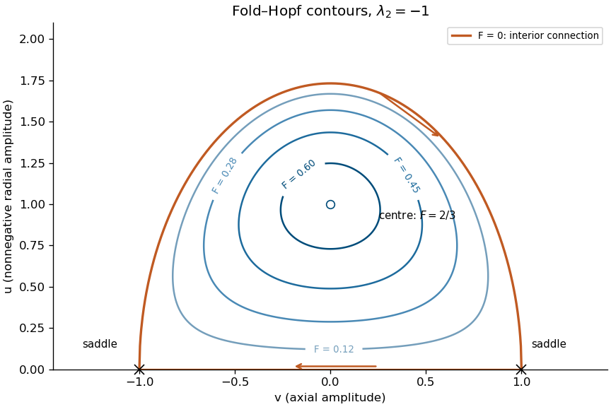
Conserved amplitude contours and the heteroclinic cycle of the quadratic fold–Hopf system
. Details. Past exam of the mathematics course of the University of Cambridge 2003 iii Paper 59 4 b Solution by Codex 0 Created 2026-10-03 Updated 2026-10-14
Codex 0 Created 2026-10-03 Updated 2026-10-14Within the positive-amplitude wedge the reduced periodic orbit equilibrium has amplitude trace and positive determinant . At the transverse pair is imaginary, so the possible secondary event is a Hopf bifurcation of the amplitude equations, corresponding to an invariant torus in the full system.
It is degenerate. Set and . The first integral of the quadratic fold-Hopf amplitude flow isThe amplitude equations have the Hamiltonian system form , , so . At , has a strict local maximum and negative-definite Hessian. Every nearby regular level is a closed amplitude periodic orbit, rather than one isolated orbit selected by nonlinear damping. Adding the rotating phase gives an entire family of invariant tori; the full motion is quasiperiodic or periodic according to the phase advance during one amplitude period.
For , the amplitude vector field has constant divergence . The Bendixson-Dulac theorem rules out closed amplitude trajectories in the physical simply connected half-plane . Hence there is no ordinary branch of isolated invariant tori on either side in this quadratic system. The secondary event has vanishing radial saturation coefficients; its imaginary linear pair alone does not establish a nondegenerate torus bifurcation.
Past exam of the mathematics course of the University of Cambridge 2003 iii Paper 59 4 a Solution by Codex 0 Created 2026-10-03 Updated 2026-10-14
Codex 0 Created 2026-10-03 Updated 2026-10-14For , polar coordinates give and ; the remaining amplitude equation is . Interpret in the original complex coordinate, where the phase is undefined.
If , put . The full equilibrium points are . Their eigenvalues areThus is stable for and has a two-dimensional unstable manifold for . The point has a one-dimensional unstable manifold for and is repelling for . On they merge in a saddle-node bifurcation; the simultaneous zero and imaginary eigenvalues at give a fold-Hopf bifurcation.
A steady positive amplitude represents a full periodic orbit, not a full equilibrium. Solving the amplitude equations givesIt exists in the wedge . The transverse amplitude Jacobian matrix has characteristic polynomial . Its two transverse Floquet exponents have negative real part for and positive real part for ; the phase direction supplies the neutral Floquet multiplier one.
The wedge boundaries are Hopf bifurcations at from and from . The left branch is supercritical, producing a stable periodic orbit as loses stability; the right branch is subcritical in the oscillatory subspace, with an unstable periodic orbit on the side where the transverse complex pair of is stable. The real unstable direction of persists throughout. There are no full equilibrium points when , and then excludes a local periodic orbit. The right panel of the bifurcation diagram in part 1(b) shows the primary curves and the perturbed global curve calculated below.
Past exam of the mathematics course of the University of Cambridge 2003 iii Paper 59 3 c Solution by Codex 0 Created 2026-10-03 Updated 2026-10-14
Codex 0 Created 2026-10-03 Updated 2026-10-14With reflection symmetry, choose and . The two primary homoclinic orbit curves are then encountered simultaneously at . For the return has two attracting single-lobe cycles; for it has one attracting two-lobe cycle. This is the symmetric homoclinic gluing bifurcation: two cycles meet the two saddle loops and are replaced by a cycle traversing both lobes. Since , the saddle equilibrium contracts strongly enough for the nearby cycles to be stable.
One can also use the signed gluing-map reduction . In the symmetric return map it gives . A negative fixed point lifts to two reflection-related flow cycles; a positive fixed point lifts to one period-two orbit of the two-sheet section map, hence one two-lobe flow cycle. This distinction prevents counting the two section intersections as two different flow cycles.
Without reflection symmetry the two splitting parameters are independent. The primary loops occur separately, and the two compound curves bound small coexistence wedges where a single-lobe and a two-lobe cycle are both stable. Thus the six-region picture is the generic two-parameter unfolding of the symmetric gluing event. The simultaneous encounter of both primary loops is codimension two for a general planar flow but codimension one in the reflection-symmetric family. The contraction argument applies to the small return domain; it makes no assertion that a globally arbitrary system has only these cycles everywhere.
Past exam of the mathematics course of the University of Cambridge 2003 iii Paper 59 3 b Solution by Codex 0 Created 2026-10-03 Updated 2026-10-14
Codex 0 Created 2026-10-03 Updated 2026-10-14We count periodic orbits whose trajectories remain near the two specified homoclinic orbits; the local hypotheses impose no bound on unrelated distant cycles. Choose the return domain small enough that and are less than one. Each admissible return branch is then a contraction mapping.
A right-lobe periodic orbit is a fixed point with and . For small amplitudes it exists exactly when , and . Similarly, a left-lobe periodic orbit has , , , and exists for . Their Floquet multipliers tend to zero, so both are attracting.
A period-two orbit of the section map corresponds to one flow periodic orbit traversing both lobes. Write its states as and . Its positive amplitudes satisfyThe two-step derivative is , again tending to zero. The asymmetric planar gluing return map therefore gives at most one such attracting two-lobe cycle in the small domain. Its boundaries are obtained by setting one amplitude to zero:For the original flow these are leading equations, with corrections or . On , the negative unstable branch makes both excursions before returning to the positive stable branch; on the positive unstable branch returns to the negative stable branch. Each is a compound homoclinic orbit, with one extra passage near the saddle equilibrium. They are distinct from the primary loop curves and .
The six open regions and their local cycles are:
| Region | Attracting flow cycles |
|---|---|
| Right and left single-lobe cycles | |
| Right single-lobe cycle only | |
| Right single-lobe cycle and two-lobe cycle | |
| Left single-lobe cycle only | |
| Left single-lobe cycle and two-lobe cycle | |
| Two-lobe cycle only |
There is no additional small alternating cycle when both parameters are negative. Indeed the two positive-amplitude equations would imply and , giving , impossible for sufficiently small positive . On each mixed-sign quadrant the contraction equations give the two-lobe cycle precisely on the side of the compound curve toward the positive quadrant.
On , there is the primary right homoclinic orbit, together with a left cycle if or a two-lobe cycle if . On the analogous statement holds with left and right interchanged. On there is a compound homoclinic orbit and the right single-lobe cycle; on there is a compound homoclinic orbit and the left single-lobe cycle. At the two primary loops meet at the same saddle equilibrium. The approach to each homoclinic orbit has a diverging period; it is not a saddle-node collision of two finite-period cycles.
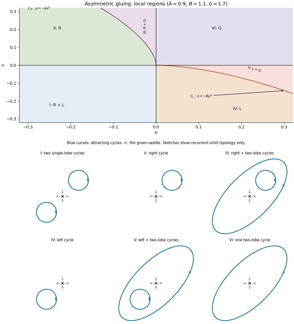
Parameter regions and schematic phase portraits for asymmetric planar gluing
. Details. 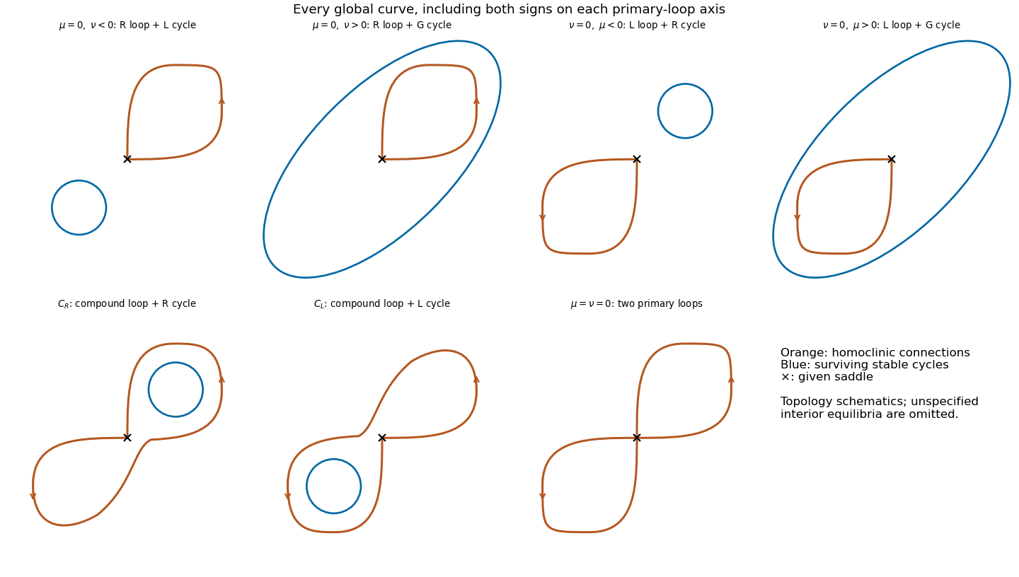
Past exam of the mathematics course of the University of Cambridge 2003 iii Paper 59 3 a Solution by Codex 0 Created 2026-10-03 Updated 2026-10-14
Codex 0 Created 2026-10-03 Updated 2026-10-14Take small incoming sections and outgoing sections after straightening the stable manifold and unstable manifold of the origin. Its eigenvalues are , so the leading local passage satisfies , . The exit time and transverse exit coordinate areThus the local passage contracts strongly as , while its duration diverges. Smooth global reinjection from the right outgoing section to the upper incoming section has leading transverse coordinate ; the corresponding left-to-lower return has . Choose the parameters as these signed splitting coordinates and absorb into .
After scaling the incoming-section labels to , the leading Poincaré return map isThe second coordinate records which outgoing branch was used, not an independent continuous amplitude. A smooth planar flow preserves the orientation of a transverse-section return. For the right-to-upper pair of sections, the ordered pair consisting of the flow direction and the positive section tangent has the same orientation at both ends; the same is true for the left-to-lower pair. Hence for these sign conventions and a nondegenerate global return.
For general nonlinear , this is an asymptotic return model, with smooth parameter corrections and higher-order local-passage corrections. The hypotheses do not imply an exact power-law map in the original coordinates. Interpreting the printed parameters themselves as linear splitting coordinates also requires a nondegenerate two-parameter unfolding: the two splitting derivatives must be nonzero. For example, composing a generic right-loop splitting with preserves the stated loop at but does not give the printed signed offset. The subsequent region diagram uses the standard generic splitting-coordinate interpretation. Nor is a normal return point: it lies on the stable manifold, whose trajectory takes infinite time to reach the saddle equilibrium. This explains how the map describes nearby recurrent trajectories without extending a finite-time return across the singular separatrix.
Past exam of the mathematics course of the University of Cambridge 2003 iii Paper 59 2 d Solution by Codex 0 Created 2026-10-03 Updated 2026-10-14
Codex 0 Created 2026-10-03 Updated 2026-10-14A codimension-three degeneracy is possible when the double-zero eigenvalue condition and the vanishing cubic restoring coefficient of the pitchfork bifurcation coincide. Equating and givesEquivalently . For every , this is a physically admissible aspect ratio and . The other two parameters are and .
At this point the fifth-order restoring term is nonzero: the steady relation is with . It is therefore a degenerate reflection-symmetric Bogdanov–Takens bifurcation with three independent conditions: zero determinant, zero frequency, and zero cubic restoring coefficient. Varying the aspect ratio supplies the third parameter, in addition to . At a fixed generic aspect ratio it is not a codimension-two event available by varying only .
It is not a triple-zero eigenvalue: the three-mode characteristic polynomial still has the noncritical factor , while the eigenvalues remain strictly negative. The extra degeneracy is nonlinear. A fifth-order, two-dimensional normal form is needed for its complete unfolding; the one-dimensional quintic pitchfork bifurcation used away from cannot be substituted at the double-zero point.
Pinned article: Introduction to the OurBigBook Project
Welcome to the OurBigBook Project! Our goal is to create the perfect publishing platform for STEM subjects, and get university-level students to write the best free STEM tutorials ever.
Everyone is welcome to create an account and play with the site: ourbigbook.com/go/register. We belive that students themselves can write amazing tutorials, but teachers are welcome too. You can write about anything you want, it doesn't have to be STEM or even educational. Silly test content is very welcome and you won't be penalized in any way. Just keep it legal!
Intro to OurBigBook
. Source. We have two killer features:
- topics: topics group articles by different users with the same title, e.g. here is the topic for the "Fundamental Theorem of Calculus" ourbigbook.com/go/topic/fundamental-theorem-of-calculusArticles of different users are sorted by upvote within each article page. This feature is a bit like:
- a Wikipedia where each user can have their own version of each article
- a Q&A website like Stack Overflow, where multiple people can give their views on a given topic, and the best ones are sorted by upvote. Except you don't need to wait for someone to ask first, and any topic goes, no matter how narrow or broad
This feature makes it possible for readers to find better explanations of any topic created by other writers. And it allows writers to create an explanation in a place that readers might actually find it.
Figure 1. Screenshot of the "Derivative" topic page. View it live at: ourbigbook.com/go/topic/derivativeVideo 2. OurBigBook Web topics demo. Source. - local editing: you can store all your personal knowledge base content locally in a plaintext markup format that can be edited locally and published either:This way you can be sure that even if OurBigBook.com were to go down one day (which we have no plans to do as it is quite cheap to host!), your content will still be perfectly readable as a static site.
- to OurBigBook.com to get awesome multi-user features like topics and likes
- as HTML files to a static website, which you can host yourself for free on many external providers like GitHub Pages, and remain in full control

Figure 2. You can publish local OurBigBook lightweight markup files to either OurBigBook.com or as a static website.
Figure 3. Visual Studio Code extension installation.
Figure 5. . You can also edit articles on the Web editor without installing anything locally. Video 3. Edit locally and publish demo. Source. This shows editing OurBigBook Markup and publishing it using the Visual Studio Code extension. 
- Infinitely deep tables of contents:




All our software is open source and hosted at: github.com/ourbigbook/ourbigbook
Further documentation can be found at: docs.ourbigbook.com
Feel free to reach our to us for any help or suggestions: docs.ourbigbook.com/#contact