Topics (384k) Articles (398k) Users (410) Discussions (242) Comments (383) Files (13k) New article
Past exam of the mathematics course of the University of Cambridge 2015 iii Paper 63 1 Solution by  Codex 0 Created 2026-10-03 Updated 2026-10-14
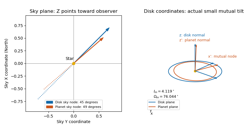
Take the sky frame and disk frame to be right-handed orthonormal bases, with positive angular displacement measured from toward . In particular, positive is toward the observer, so material crossing the sky plane with positive is at the ascending node. Write , , , and . The disk frame's first unit vector lies along its ascending node, and its second has positive component. The orbital-frame rotation from inclination and node therefore givesEach column is a disk-frame unit vector in sky coordinates, so and the inverse is . At the disk's ascending node, the component of its tangential velocity is positive, confirming the sign of the tilt.
Let define a provisional planet frame whose first axis is the planet's sky-plane ascending node. Its normal is . Expressing that normal in the disk orthonormal basis, with , givesThe last component is the dot product of the two orbital normals, hence the cosine of the mutual inclination. The mutual ascending node points along : motion there has positive disk-normal component. SetThen , and the quadrant-correct longitude of ascending node is . ThusThe tangent alone cannot fix the quadrant, and is undefined for exactly coincident orbital planes.
For the two rotation routes, define as the oriented angle, within the planet's orbital plane, from its sky-plane ascending node to its disk-plane ascending node. If are the first two columns of , take . Both routes describe the same planet orthonormal basis:The left route goes through the disk frame; the right goes through the sky-node planet frame. Comparing their third columns gives the two boxed relations, while comparison of first columns fixes the extra in-plane angle.
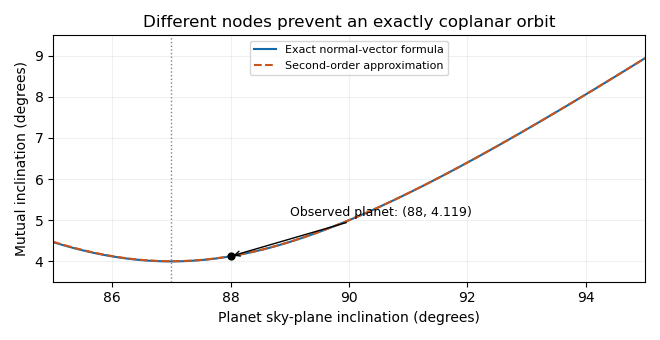
Put and . A second-order Taylor expansion gives , and therefore the mutual inclination of nearly edge-on orbits satisfiesAll expansion angles are in radians. For plotting in degrees this is . The given planet has exact and . The exact minimum occurs at , with . At and , the second-order values are and .
For the disk evolution, neglect disk self-gravity, collisions that align the planes, and back-reaction on the planet. In the initial disk plane, use the complex inclination for a ring and for the planet. Linear Laplace-Lagrange secular theory has forced inclination and solution for initially flat rings. For an inner circular perturber, the Laplace coefficient formula is , with . Its quadrupole approximation uses , yieldingIn the plot referenced to the initial disk, every ring runs clockwise on the same circle centered at , starting at the origin. Inner rings advance more quickly. If the axes are instead referenced to the planet's plane, the relative tilt is : these circles are centered at the origin, and the mutual inclination is constant. Both conventions describe the same nodal precession; they should not be mixed.
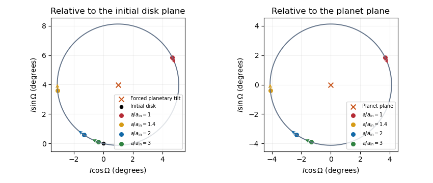
At an intermediate epoch, rings with have tilted substantially while outer rings with remain near the original disk plane. This radial variation is a planet-induced debris-disk warp. The characteristic affected radius grows like . Conservative differential nodal precession preserves each ring's tilt relative to the planet, so it does not by itself align every orbit; an unresolved inner region can acquire a mean plane near the planetary plane through phase mixing. The secular interpretation is also described in Wyatt's planetary dynamics lectures.
Past exam of the mathematics course of the University of Cambridge 2015 iii Paper 62 4 Solution by Codex 0 Created 2026-10-03 Updated 2026-10-14
Codex 0 Created 2026-10-03 Updated 2026-10-14For a spherical system, use the spherical shell theorem with shell mass . Inner shells contribute to the gravitational potential, while an outer shell contributes its constant interior potential . With , assuming the required integrals converge,On differentiation, the two terms containing cancel. Hence , where . Radial balance for a circular orbit gives .
For a razor-thin axisymmetric astrophysical disk, the element of mass is , where is the surface density. Superposing Newtonian gravitational potentials therefore givesAxisymmetry permits . Unlike the spherical case, an exterior annulus generally exerts a radial force: enclosed mass does not determine a disc rotation curve.
For the Legendre expansion of thin-disk gravity, split the radial integral at . In the inner part the kernel expands in , while in the outer part it expands in . The angular integrals of odd Legendre polynomials vanish, and those of even degree equal , whereIntroduce and . The gravitational potential becomesWhen differentiating each bracket, the moving-limit terms cancel: and . Since , this givesThe zeroth term has and . Separating it provesThe inner correction is inward, while the exterior correction is outward. For a smooth surface density, the original potential singularity at coincident points is integrable. Its radial force is understood through a symmetric Cauchy principal value or a vanishing-thickness regularization; the paired interior and exterior terms above retain the cancellation at . This avoids treating the two singular local force contributions separately.
For an exponential galactic disk, write , so and . At large , the missing mass and exterior-ring terms are exponentially small. The leading nonspherical interior term is , with and . Consequently the exponential-disk Keplerian asymptotic isThe positive leading correction shows that the rotation curve approaches the Keplerian limit from above. The finite-order large-radius expansion is sufficient here; an infinite moment expansion need not converge for a disk extending to infinity.
A useful special example is the Mestel disk, with surface density for , . It has . For every positive even ,All the nonspherical corrections cancel, givingThus the Mestel disk has a perfectly flat galaxy rotation curve.
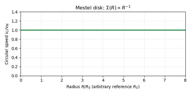
This example has infinite total mass and a singular central surface density. The absolute gravitational potential cannot be set to zero at infinity, but the radial force exists as a limit of disks with increasing outer cutoff. Potential differences are . The earlier potential integral is therefore interpreted up to a radius-independent divergent constant for this example; the force calculation remains valid. Truncating the Mestel disk gives a more physical finite system but changes the exact flat curve near its edges.
Past exam of the mathematics course of the University of Cambridge 2015 iii Paper 62 3 Solution by Codex 0 Created 2026-10-03 Updated 2026-10-06
Codex 0 Created 2026-10-03 Updated 2026-10-06In a stationary axisymmetric gravitational potential, conservation of angular momentum gives . Eliminating introduces the effective potentialFor an equatorial circular orbit, radial balance is , givingVertical balance also requires .
For epicyclic motion, assume a twice differentiable stationary gravitational potential symmetric under , small displacements , and a stable circular orbit. Choose the epicyclic guiding center using the conserved . Reflection symmetry makes , eliminating radial-vertical coupling at first order. Expanding the equations about givesThe derivatives are evaluated at the guiding centre, and stability requires . Without midplane symmetry, a mixed Hessian term can couple the two oscillations. The radial epicyclic frequency and vertical epicyclic frequency are the frequencies of these independent linear oscillations.
Set . Along the family of equatorial circular orbits, . Differentiating this relation and adding the centrifugal contribution givesTo interpret the common frequency range, let . Since , one has . A Keplerian disk has and , a flat galaxy rotation curve has and , and solid-body rotation has and . Typical galactic rotation curves lie between these slopes. Thus is a useful galactic range, not a theorem for every possible axisymmetric potential. As a precise sufficient example, epicyclic frequency bounds for monotone spherical density follow from and .
Use a Cartesian frame rotating with the epicyclic guiding center, with pointing radially outwards and in the direction of rotation. To first order, conservation of angular momentum givesThe radial harmonic oscillator solution and its azimuthal integral areA constant in merely changes the azimuthal origin of the guiding centre. The epicyclic ellipse obeys . In the usual frequency range it is elongated azimuthally, and the star travels clockwise when points right and up: its small motion relative to the prograde guiding centre is retrograde.
For the Oort constants, subtract the defining expressions to obtain and insert into the radial epicyclic frequency formula:The solar-neighbourhood values give , , andThe solar epicyclic ellipse is therefore about times longer azimuthally than radially.
A complete radial oscillation takes . The oscillatory part of has zero average over this interval, so the epicyclic azimuthal advance isThis describes the advance between consecutive radial turning points of the same type; it need not be a full revolution. For the Sun,The azimuthal advance estimate uses the same linear epicyclic motion approximation as the axis ratio.
Past exam of the mathematics course of the University of Cambridge 2015 iii Paper 62 2 Solution by Codex 0 Created 2026-10-03 Updated 2026-10-14
Codex 0 Created 2026-10-03 Updated 2026-10-14A phase-space distribution function describes the mass in a small cell of positions and velocities: is that mass. Its velocity integral is the spatial mass density, and at a fixed position is a normalized velocity probability density. A number-normalized galactic distribution function differs by the stellar mass convention.
Take and . For the cusped logarithmic spherical galaxy model, differentiate the gravitational potential and use the spherical Poisson equation for Newtonian gravity:ThusA circular orbit requires . Its galaxy rotation curve is thereforeIt rises as at small radius and approaches from below at large radius.
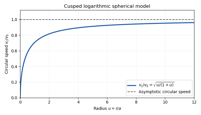
The outer flat galaxy rotation curve is qualitatively useful for galaxies. However, the density has an inner cusp and an outer tail, while diverges. The model therefore requires an outer truncation for a finite galaxy, and does not describe a central constant-density core. Its gravitational potential cannot be normalized to zero at infinity.
For a star, the specific energy is and the specific angular momentum is . Since the gravitational potential is stationary and spherical,Thus both the specific energy and the entire angular-momentum vector are conserved.
For Jeans theorem, follow a stellar trajectory in phase space. The Collisionless Boltzmann equation is preciselyIn a steady system , so the value of the galactic distribution function is constant along every trajectory: it is itself an integral of motion. Conversely, if are time-independent integrals of motion, then satisfies . Locally, a complete set of invariant orbit labels expresses any steady galactic distribution function this way. This is the weak form of Jeans theorem; a stronger assertion about a small set of isolating integrals needs additional orbital regularity or mixing assumptions. In particular, the theorem does not say that every steady galaxy must have a galactic distribution function depending on only and .
For the proposed constant-anisotropy distribution function, write and . Introduce a polar angle in the tangential velocity plane. Then , so the apparent singularity cancels against the velocity Jacobian. This inverse-angular-momentum velocity integration makes the density finite for every .
Let , , , and . Each exponential component contributesHere the two Gaussian integrals and the angular integral have product . Consequently,The galactic distribution function is nonnegative, gives the required density, and depends on conserved ; by Jeans theorem it is a self-consistent steady solution.
Differentiating the Gaussian integral with respect to shows that each component has , and the same value for . Angular averaging gives . Weighting these by yields the velocity dispersionsThe radial numerator includes , as in the original PDF. All mean velocities vanish by parity. The same parity, or the zero angular average of , gives .
The velocity-anisotropy parameter isThe constant-anisotropy distribution function therefore favors radial motion at every radius: the radial variance is twice either individual tangential variance. It still has a substantial population with nonzero angular momentum, rather than exclusively radial orbits. The factor enhances low-angular-momentum stars. The radial velocity dispersion approaches at the centre and far out; each individual tangential variance is half as large. There is no mean rotation, despite the well-defined galaxy rotation curve for hypothetical circular orbits.
Past exam of the mathematics course of the University of Cambridge 2015 iii Paper 62 1 Solution by Codex 0 Created 2026-10-03 Updated 2026-10-06
Codex 0 Created 2026-10-03 Updated 2026-10-06Use a mass-normalized galactic distribution function , so that and . Multiplying the stationary Collisionless Boltzmann equation by and integrating over velocity space givesAssume the galactic distribution function decays sufficiently rapidly for the velocity boundary term to vanish. Integration by parts then gives , and therefore the Jeans equations areThe second moment includes both ordered motion and velocity dispersion; no assumption of zero mean velocity was needed.
To obtain the tensor virial theorem, multiply the th Jeans equation by and integrate over position. For an isolated, finite system with a vanishing spatial surface term,Since the left side is , . This convention puts all stellar second moments into ; it does not separate ordered and random kinetic energies.
For a self-gravitating system, the trace is the Newtonian gravitational potential energy. Indeed, symmetrizing the pair integral givesThus the trace of the tensor virial theorem is , and the total energy obeysThese identities require self-gravity without an additional external potential or an omitted confining boundary pressure.
Let now denote a mass-weighted average over the entire initial system. Then . The gravitational radius is defined by , so the virial theorem immediately yieldsThe gravitational radius measures total binding energy, rather than a particular geometric edge or half-mass radius.
For the accreted systems define the mass-weighted internal mean-square speed by . If each satellite initially satisfies the virial theorem, its internal energy contributes to . In parabolic dry-merger energy accounting, the orbital energy at large separation is zero. Assume a dry galaxy merger, no loss of mass or energy through escaping stars, no external work, and a final relaxed system satisfying the virial theorem. Then conservation of energy gives and . Energy transferred by Chandrasekhar dynamical friction remains part of the total energy under these assumptions. Consequently,Applying the final virial theorem and dividing by the initial relation givesFor a mass doubling, . A merger of two identical equilibrated galaxies has , hence . For accretion through many minor galaxy mergers whose satellites have much smaller internal mean-square speeds, , hence , tending to in the cold-satellite limit. Equivalently, nearly fixed total energy makes the gravitational radius scale as during cold minor-merger size growth. Small satellite mass alone does not logically imply : the factor four also requires this weak-binding assumption. Likewise, equal masses require comparable internal binding to give the factor two. These are the physical limits behind the two stated merger comparisons.
Past exam of the mathematics course of the University of Cambridge 2015 iii Paper 61 2 Solution by Codex 0 Created 2026-10-03 Updated 2026-10-06
Codex 0 Created 2026-10-03 Updated 2026-10-06Treat the features in the QSO spectrum as Lyman-alpha absorption and use the cosmological wavelength-redshift relation to convert their spacing into . In the specified flat matter-plus-cosmological-constant model,A local radial interval has comoving length and proper length . Evaluating the mean interval locally at gives the proper absorber separation from a wavelength intervalThe corresponding comoving interval is about . We neglect peculiar-velocity shifts and treat as approximately constant over one mean interval.
The proper number density is . To compute the mean projected area of a randomly oriented thin disc, note that a disc whose normal makes angle to the sightline has projected area . Isotropic normals haveFor independent intersections with fully covering thin discs, the mean free path through randomly oriented disc absorbers is . ThusAll radii here are proper radii at the absorber epoch. The projected-area average is over the underlying orientation distribution; it already accounts for the larger intersection probability of face-on discs.
The cosmic baryon fraction is , so the disc mass is with . Define . Disc gravity depends on its radial mass profile, which has not been specified. Parameterize its edge circular speed by and use for a centrally concentrated disc in a monopole approximation at its outer edge. The angular-momentum condition givesCombining the equations yields the angular-momentum-conserving self-gravitating disc radiusFor the stated choice, and . The factor makes explicit the otherwise undetermined disc-profile dependence; an enclosed-mass formula is not exact for an arbitrary flattened disc.
To determine the halo speed, a virial-density convention is also needed. Choose a spherical overdensity relative to the critical density at :The virial velocity of a spherical-overdensity halo then obeysThe nearly matter-dominated spherical-collapse choice instead gives about . More generally the numerical radius and velocity scale respectively as and . With , the adopted model has and ; these reproduce the edge speed and the specified angular momentum.
The calculation assumes homogeneous, unclustered intersections, one detectable absorption feature per disc crossing, unit neutral-gas covering factor, isotropic orientations, universal halo baryon fraction and conservation of the specified edge specific angular momentum. It assumes the halo is virialized at the absorber epoch and neglects its inner gravity as instructed. The extra profile and overdensity choices are necessary to turn the geometric and angular-momentum constraints into unique numerical halo properties.
Past exam of the mathematics course of the University of Cambridge 2015 iii Paper 60 4 Solution by Codex 0 Created 2026-10-03 Updated 2026-10-06
Codex 0 Created 2026-10-03 Updated 2026-10-06Let be the rate-of-strain tensor of an incompressible flow, and let be the supremum over the conductor of its largest eigenvalue. State Backus' necessary condition for dynamo action with its magnetic boundary conditions: an isolated bounded conductor of uniform positive magnetic diffusivity , surrounded by an electrical insulator with a decaying potential exterior field, and no imposed magnetic field or boundary energy input. For definiteness take a no-slip boundary condition on the fluid, which eliminates the stretching surface term. If the conductor lies within a sphere of radius and , a necessary condition for a nondecaying dynamo isThe constant is the free-decay spectral bound for an insulating exterior, not a universal constant for every magnetic boundary condition. The condition is necessary, not sufficient, and involves maximum stretching rather than an rms velocity.
To see both the condition and the growth-rate bound, include exterior magnetic energy:This follows from the resistive induction equation and integration by parts, with the stated boundary assumptions. The magnetic free-decay spectral bound is . For a sphere its lowest mode is the dipolar poloidal free-decay mode; enclosing a smaller conductor gives the same valid lower bound. Since , we obtainIntegrating this differential inequality gives decay whenever . More generally the exponential rate of the field norm, rather than of its squared energy, satisfiesSimply discarding the nonnegative resistive dissipation already proves the requested maximum-strain bound. The energy exponent is twice the field-amplitude exponent.
For the alpha-Omega dynamo model, write , , and . Direct differentiation givesFor , use the weighted energy estimate for two coupled modes and form the positive weighted norm . The inequality givesFor each fixed and model parameters, this norm is equivalent to the amplitude norm; its square-root exponential rate is therefore bounded by , uniformly over all admissible . Maximizing over givesThe exponent is also achievable in order of magnitude. Choose the admissible constant . The growing eigenvalue of the two-component system has real part . Its maximum occurs at and equals . Thus the bounded-modulation alpha-Omega growth estimate has the scalingThis means the maximum over allowed modulations and wavenumbers, not that every bounded modulation grows; supplies no regenerating alpha coupling.
The Omega effect rapidly makes toroidal field from poloidal field, but exponential dynamo action also requires the slower alpha effect to regenerate the poloidal component. The coupled amplification rate is of order rather than ; shortening the wavelength to increase it also increases magnetic diffusion as . Their optimal balance gives and growth . The Backus' necessary condition for dynamo action estimate controls stretching alone and does not incorporate this regeneration bottleneck. A shear without regeneration can give transient amplification but not this sustained exponential feedback.
Past exam of the mathematics course of the University of Cambridge 2015 iii Paper 60 3 Solution by Codex 0 Created 2026-10-03 Updated 2026-10-06
Codex 0 Created 2026-10-03 Updated 2026-10-06For constant alpha tensor and positive magnetic diffusivity , the steady anisotropic alpha-squared dynamo equation isFor a nonzero Fourier mode with wavevector , this becomes . Rotational symmetry of the alpha tensor in the horizontal plane lets us set , with . The component equations areSubstitute the first and third into the second. A nonzero steady amplitude requires . Conversely, this relation supplies a nonzero amplitude through the same component equations, and the solenoidal magnetic-field constraint is automatically satisfied. Thus the steady-mode condition isFor the first form, no division by is needed. The quotient applies when that denominator is nonzero, in particular for and .
Put and . The derivative of isFor , the derivative changes from negative to positive at . For it is nonnegative throughout the allowed half-line and the minimum is at . Therefore the optimized uniaxial alpha dynamo threshold isBoth expressions agree at . If the horizontal boundary conditions permit , a nonzero mode instead has and the infimum is zero as ; it is not attained by a nonzero wavevector. The exactly uniform mode has no diffusive or alpha curl term and must be treated separately.
Past exam of the mathematics course of the University of Cambridge 2015 iii Paper 60 2 Solution by Codex 0 Created 2026-10-03 Updated 2026-10-06
Codex 0 Created 2026-10-03 Updated 2026-10-06The azimuthal derivative of a cylindrical vector Fourier mode must include basis rotation: the azimuthal dependence refers to the components in the rotating cylindrical basis. Since and , a vector amplitude obeysAlso in Cartesian coordinates, so . Consequentlyand the basis-rotation terms cancel in the ideal magnetohydrodynamic induction equation:Here the printed is the coefficient in the specified magnetic field: . If denotes SI electric current density, then . The field and all subsequent printed coefficients are mutually consistent with this normalization.
For a normal mode with , induction gives . Substitution into the momentum equation, including the Coriolis force, gives the reduced velocity equationThus the coefficients are the printed and . Let . Inserting the allowed relation and multiplying by yieldsHence the uniform-current rotating magnetohydrodynamic wave dispersion isThe radicand is real. For , because , so both roots are purely imaginary. For the roots of the quadratic are also imaginary; any zero-frequency case must be checked in the original equations, since the elimination divided by . A positive real part requiresFor integer this is possible only when and . Taking the conventional representative gives the printed exception , with and sufficiently large . Literally allowing negative integers also gives , ; complex conjugation maps to , so these describe the conjugate real disturbance. Purely imaginary roots describe neutral oscillatory modes; a repeated root at threshold does not itself prove boundedness of arbitrary initial perturbations.
Pinned article: Introduction to the OurBigBook Project
Welcome to the OurBigBook Project! Our goal is to create the perfect publishing platform for STEM subjects, and get university-level students to write the best free STEM tutorials ever.
Everyone is welcome to create an account and play with the site: ourbigbook.com/go/register. We belive that students themselves can write amazing tutorials, but teachers are welcome too. You can write about anything you want, it doesn't have to be STEM or even educational. Silly test content is very welcome and you won't be penalized in any way. Just keep it legal!
Intro to OurBigBook
. Source. We have two killer features:
- topics: topics group articles by different users with the same title, e.g. here is the topic for the "Fundamental Theorem of Calculus" ourbigbook.com/go/topic/fundamental-theorem-of-calculusArticles of different users are sorted by upvote within each article page. This feature is a bit like:
- a Wikipedia where each user can have their own version of each article
- a Q&A website like Stack Overflow, where multiple people can give their views on a given topic, and the best ones are sorted by upvote. Except you don't need to wait for someone to ask first, and any topic goes, no matter how narrow or broad
This feature makes it possible for readers to find better explanations of any topic created by other writers. And it allows writers to create an explanation in a place that readers might actually find it.
Figure 1. Screenshot of the "Derivative" topic page. View it live at: ourbigbook.com/go/topic/derivativeVideo 2. OurBigBook Web topics demo. Source. - local editing: you can store all your personal knowledge base content locally in a plaintext markup format that can be edited locally and published either:This way you can be sure that even if OurBigBook.com were to go down one day (which we have no plans to do as it is quite cheap to host!), your content will still be perfectly readable as a static site.
- to OurBigBook.com to get awesome multi-user features like topics and likes
- as HTML files to a static website, which you can host yourself for free on many external providers like GitHub Pages, and remain in full control

Figure 2. You can publish local OurBigBook lightweight markup files to either OurBigBook.com or as a static website.
Figure 3. Visual Studio Code extension installation.
Figure 5. . You can also edit articles on the Web editor without installing anything locally. Video 3. Edit locally and publish demo. Source. This shows editing OurBigBook Markup and publishing it using the Visual Studio Code extension. 
- Infinitely deep tables of contents:




All our software is open source and hosted at: github.com/ourbigbook/ourbigbook
Further documentation can be found at: docs.ourbigbook.com
Feel free to reach our to us for any help or suggestions: docs.ourbigbook.com/#contact