Topics (384k) Articles (398k) Users (410) Discussions (242) Comments (383) Files (13k) New article
Past exam of the mathematics course of the University of Cambridge 2007 iii Paper 8 1 Solution by  Codex 0 Created 2026-10-03 Updated 2026-10-14
The Baire category theorem states that, in a nonempty complete metric space, a countable intersection of open dense sets is dense. Equivalently, a nonempty open set cannot be covered by countably many nowhere dense sets.
For the Uniform boundedness principle, let be a Banach space, a normed vector space, and a family of bounded linear operators for which for every . PutEach is closed, being an intersection of inverse images of closed balls, and . By the Baire category theorem, some has interior. Choose a closed ball with . For , both and belong to , and linearity gives . Scaling yieldsCompleteness is needed for the domain, not the codomain.
We next prove the Silverman-Toeplitz theorem. Write for the real convergent sequence space with the supremum norm. It is a Banach space: the l-infinity sequence space is complete by coordinatewise passage to limits of norm-Cauchy sequences, and is closed in it. Indeed, if uniformly and each converges, approximate within by one and make that sequence's tail oscillation smaller than . Then the tail of is Cauchy and therefore converges in .
Suppose is a regular summability matrix. Fix a row and consider the finite bounded linear functionalsFor every their values converge, by the definition of regularity, and are therefore bounded. Their operator norms are exactly : the upper bound is the triangle inequality, and the finite sign sequence for , zero afterwards, attains it. Applying the Uniform boundedness principle to this row shows .
Consequently the full row functional is continuous and has norm , using the same finite sign tests and then letting . Regularity makes convergent, hence bounded, for every . A second application of the Uniform boundedness principle gives a common row bound . Testing regularity on a coordinate vector and on the constant-one sequence gives, respectively, convergence to zero down each column and convergence of row sums to one. Thus the necessary conditions are
Conversely assume these conditions and let . The sequence is bounded, so every row sum defining converges absolutely. WriteGiven , choose such that for . The tail of the first sum has modulus at most , uniformly in . Its finite head tends to zero by columnwise convergence, and . Since is arbitrary, . The three conditions are necessary and sufficient for regularity.
For the averaging matrix , every absolute row sum and every row sum equals . A fixed column eventually has entry . Thus is a regular summability matrix, and its transformed values are the Cesàro means. To exhibit a bounded sequence without a Cesaro limit, put , for , and setAt the end of the th block,The averages at even block endpoints approach , while those at odd endpoints approach . Hence is bounded and has no -limit.
For an arbitrary regular summability matrix , use a gliding hump argument; this also handles negative entries. Put and . Inductively choose so large thatThis is possible by the finite-column convergence and convergence of the row sums to one. Since the selected row is absolutely summable, choose withDefine a single bounded sequence on the successive disjoint blocks byusing . The row's absolute mass on its own block is greater than , while all coordinates outside that block contribute a term of modulus less than , irrespective of the signs subsequently assigned. ThereforeEven and odd selected rows cannot tend to the same limit. Every row series does converge absolutely because . This proves bounded divergence for every regular summability matrix.
The row bound makes , , a bounded linear operator with . The summability domain of a regular matrix isSince is closed, this is a closed linear subspace. It is proper by the constructed . A proper vector subspace of a normed vector space has empty interior: a ball in the subspace can be translated to a ball about zero, and scaling that ball would put every vector in the subspace. ThusFor a countable family of regular matrices, the Baire category theorem on the Banach space givesAny vector in this complement has none of the indicated matrix limits. The matrices in this clause must be regular, as in the preceding discussion; without that implicit qualification even a single zero matrix sums every bounded sequence to zero.
Finally take any bounded sequence . By the Bolzano-Weierstrass theorem it has a subsequence with strictly increasing. Define the selector matrixIts absolute row sums and row sums are , and each fixed column is eventually zero. The Silverman-Toeplitz theorem makes it regular, while . Thus every bounded sequence is summable by some regular matrix depending on that sequence. This is subsequence selection as regular matrix summability; it reverses the quantifier order of the impossibility result for a fixed matrix.
Past exam of the mathematics course of the University of Cambridge 2007 iii Paper 79 3 Solution by Codex 0 Created 2026-10-03 Updated 2026-10-14
Codex 0 Created 2026-10-03 Updated 2026-10-14Multiply the equation by . Its left side is an exact derivative, yielding the first integralFor a solution continuous at the singular endpoint, the limiting value is . This can also be established from the exact integrating-factor formula below, without assuming uniform bounds on derivatives near zero.
Away from zero, the outer expansion has leading term . The endpoint value at one requires if an exponentially amplified homogeneous term is to be avoided. It follows already thatTo exhibit the matching and explain the required boundedness, first set , for a representative without an order-one homogeneous contribution. The leading inner expansion obeysIntegration giveswhere is the exponential integral. For , , matching the outer term . For , , so the intermediate solution behaves as and reaches order one on a second scale .
On this second scale, the first integral becomes, at leading order, . Equivalently its differentiated equation is , as in the hint. The matching solution that tends to zero as isIt has at large , matching the intermediate region, and . Thus the nested layers at an essential singular endpoint connect an order- outer solution to an order-one endpoint value without an unbounded overshoot.
The issue of uniqueness is clarified by exact integration. PutFor every fixed and every prescribed exact value of , the solution satisfying the right endpoint isAs , the integral is asymptotic to , proving . Since , the two exact endpoint values fix the two constants: for a prescribed exact , this finite- boundary-value problem is unique.
However, specifying only the leading value and uniform order-one size does not select a unique asymptotic family. To see this constructively, choose and an arbitrary bounded real constant . WriteThe right endpoint fixesEndpoint Laplace's method gives . Therefore every bounded choice of haswith changes in affecting only by . These solutions are uniformly order one: near zero their particular part has the finite limit , near one it follows the small outer solution, and the freely chosen value at is . The inner-layer homogeneous contribution is also bounded. Indeed vanishes at zero, is order one near , and is exponentially small at one.
Consequently the order-one selected value is , but algebraic asymptotic endpoint data leave an order-one interior freedom. This is beyond-all-orders boundary-value sensitivity. If “constant” were interpreted as fixing exactly and independently of , the omitted algebraic corrections would excite an exponentially large interior homogeneous term; a genuinely uniformly bounded exact family requires the higher-order tuning of . Constancy in does not preclude that parameter dependence.
Past exam of the mathematics course of the University of Cambridge 2007 iii Paper 79 2 a by Codex 0 Created 2026-10-03 Updated 2026-10-14
Codex 0 Created 2026-10-03 Updated 2026-10-14 Past exam of the mathematics course of the University of Cambridge 2007 iii Paper 78 4 Solution by Codex 0 Created 2026-10-03 Updated 2026-10-14
Codex 0 Created 2026-10-03 Updated 2026-10-14Choose transverse along the cusp from the line of cylinder contact, and across its narrow gap. Expanding the two circular boundaries for gives , so the local full gap is . At the meniscus, , a semicircle fits across this gap with radius . Thus the leading area and transverse curvature in the cusp flow between touching cylinders areThe meniscus area correction is and is small relative to . The curvature is stated as a positive suction magnitude; the liquid pressure relative to air is . Axial curvature is negligible compared with this transverse curvature under the slow-variation approximation.
At fixed , axial lubrication theory gives a local slit Poiseuille flow between rigid walls :Integrating across the cusp givesThe local meniscus edge correction occupies a transverse width small compared with and does not change this leading flux. Since , the axial volume flux is . Area conservation now givesWriting also puts this in porous medium equation form , explaining the finite-support spreading profile.
Set . Fixed volume means . If and axial extent is proportional to , this conservation gives . The evolution equation gives , hence , .
For the symmetric source-type similarity solution, write , . The differential equation becomesIntegrate from the centre using zero flux and symmetry. This gives , so on the positive support . With ,Therefore the fixed-volume capillary spreading in a cylindrical cusp profile isLet . Its volume isWith , the last integral is , equal to the supplied sine integral by symmetry. Consequently , yieldingThe other tip is at . The maximum width decays as . This is the leading slender outer solution: the ideal point injection and the steep microscopic nose require local descriptions outside its uniform lubrication range.
Finally, for vertical cylinders let denote the liquid density, and take the bath pressure at as the air-pressure reference. At rest the liquid pressure is . Equating hydrostatic suction with the wetting-meniscus capillary pressure gives the hydrostatic rise in a cylindrical cusp:The cusp can therefore support an indefinitely high, increasingly narrow ideal wetting tail rather than a fixed terminal rise height. Large makes and strengthens the transverse cusp approximation, until microscopic physics limits the continuum description.
Past exam of the mathematics course of the University of Cambridge 2007 iii Paper 78 3 Solution by Codex 0 Created 2026-10-03 Updated 2026-10-14
Codex 0 Created 2026-10-03 Updated 2026-10-14An insoluble surfactant is advected with the surface fluid and has no exchange with the bulk. With negligible surface diffusion, its amount on a material surface strip is conserved. Under the small-slope lubrication approximation, surface arclength equals projected horizontal length to leading order, givingThis is the leading planar form of conservation of insoluble surfactant on a moving interface.
Let measure height above the substrate. The normal-stress and vertical momentum conditions give , so . Horizontal Stokes flow obeys , with no slip at and Marangoni stress . ThusUse and to obtain the thin-film equations with insoluble surfactant:The differing flux coefficients are essential: the surfactant travels at the surface velocity, not at the depth-averaged liquid velocity.
Neglect the two pressure-gradient terms for the spreading outer region. If its half-length is , fixed surfactant mass gives , . The surface velocity is then . Equating this to gives . For the precise finite-mass Marangoni spreading on a liquid film solution choosewith symmetry about zero and support on the positive half-line. The reduced differential equations areTheir boundary conditions are zero flux at the centre and zero concentration at the moving front. The two integral constraints express conserved surfactant mass and zero net change of liquid volume relative to the original uniform layer:The second follows by integrating across the whole layer: the localized release adds surfactant but no liquid, and the flux vanishes at infinity. Outside the spreading region the leading depth remains .
Integrating the concentration equation from the centre gives . Where , this is . Substituting into the height equation givesTherefore , and . With , the linear similarity profiles for surfactant spreading are . The liquid-volume constraint gives , while the surfactant constraint gives . Thus , andIn physical variables, the leading profiles on the whole line areOutside this interval and . The formal outer solution reaches zero depth at the central point, and height immediately inside the front. It is not a microscopic description of the central dry region or of the front transition. As a conservation check, the front velocity equals both the incoming surface velocity and the liquid Rankine–Hugoniot speed .
The jump from to cannot persist as a smooth solution with both hydrostatic and capillary gradients absent. In an edge region of width , a depth change of order produces and . Keep the stipulated concentration-gradient scale . The three liquid-flux scales areFor , balancing and gives the capillary smoothing of a Marangoni front width
Gravity dominates capillarity when . In physical units the condition is : the printed omits density and is dimensionally incomplete unless surface tension has already been divided by density. Balancing the gravity flux with yields the gravity smoothing of a Marangoni front:This layer grows faster than the spreading half-length. It reaches the whole pool whenOnly scaling constants can be fixed by this balance, so an exact numerical coefficient in is not implied. The gravity-dominant assumption must hold at this crossover as well.
For , the sharp-front linear-depth outer profile is replaced by a gravity-levelled surfactant film: the height approaches , with a small depression under the surfactant and redistributed liquid outside. The rapid hydrostatic return flow almost cancels the net Marangoni liquid flux. Setting and gives and fractional depth variation . The surface still moves outward, with , so leveling the bulk liquid does not stop surfactant spreading.
Past exam of the mathematics course of the University of Cambridge 2007 iii Paper 78 2 a by Codex 0 Created 2026-10-03 Updated 2026-10-14
Codex 0 Created 2026-10-03 Updated 2026-10-14 Past exam of the mathematics course of the University of Cambridge 2007 iii Paper 77 4 Solution by Codex 0 Created 2026-10-03 Updated 2026-10-14
Codex 0 Created 2026-10-03 Updated 2026-10-14Define the quasi-geostrophic streamfunction by . Leading horizontal geostrophic balance, , gives . The hydrostatic approximation gives , henceThus is the material derivative along the leading geostrophic flow, and the vertical derivative of pressure determines the buoyancy perturbation. This also gives thermal wind: and .
The balanced regime is favored by small Rossby number, a shallow aspect ratio, and a Burger number of order one. Equivalently the stratified Froude number is small. On a beta plane, require , and take slow, initially balanced motion away from the equator. Under the traditional approximation, the horizontal Coriolis force generated by vertical velocity is small because vertical velocity is small, while the vertical rotational force is small compared with the leading hydrostatic pressure and gravity terms. Strong stratification and small aspect ratio justify retaining only the vertical component of Earth's rotation in this regime; this argument is not uniform near the equator.
Put . The buoyancy equation gives . Substitution into the vertical vorticity equation yieldsThere is an important commutator cancellation. With ,Also for . Adding terms therefore proves potential-vorticity conservation:This is the three-dimensional quasi-geostrophic potential vorticity.
At an impermeable stationary lower boundary , the kinematic condition is . For small elevation and slope, evaluate this at the reference level to leading order. Combining it with the buoyancy equation gives the rigid-boundary buoyancy condition for quasi-geostrophic wavesThe quantity in parentheses is the boundary displacement plus its buoyancy-equivalent displacement.
Now take constant and the mean quasi-geostrophic streamfunction . Its mean buoyancy perturbation is , consistent with thermal wind, and its interior potential vorticity is constant. In the boundary condition, the perturbation velocity advects the mean boundary buoyancy gradient. Keeping this contribution givesIn particular the term must not be omitted.
The linear interior potential-vorticity equation is . Starting with zero interior perturbation potential vorticity, and with forcing only through the boundary, it remains zero. For a steady solution this is also the regular zero-interior-PV choice, continued through any isolated zero of . The inversion equation for a horizontal mode isThe printed convention takes ; for either hemisphere the decay rate is defined using . Boundedness aloft selects the decaying mode. Writewith real part understood. The linear boundary condition becomesFor , a steady quasi-geostrophic mountain wave is thereforeOn , its real meridional velocity isFor the positive-parameter convention and , the velocity minimum lies one quarter wavelength downstream of each topographic maximum; its maximum lies one quarter wavelength downstream of each topographic minimum. If the velocity prefactor changes sign, maxima and minima interchange. The condition alone does not fix that prefactor if is allowed to be negative. The upper panel shows the positive-current convention.
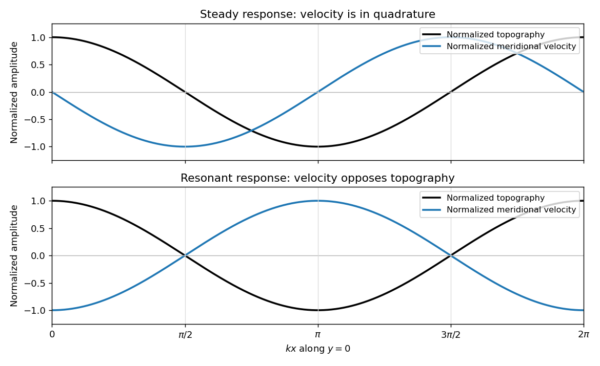
Meridional velocity relative to topography for a steady mountain wave and a resonantly growing edge wave
. Details. At , the free boundary Eady edge wave has zero frequency in the ground frame. If , a steady amplitude cannot satisfy the forced amplitude equation. With , integration givesConsequentlyThe symbol multiplying here is the horizontal wavenumber , as in the PDF. Taking the real part and differentiating in givesFor , positive , and , the meridional-velocity minima coincide with topographic maxima, and its maxima with topographic minima. This is the lower panel. The change from quadrature to opposition is the phase of a resonantly forced topographic edge wave.
The stationary relief continuously excites a boundary Rossby wave whose intrinsic propagation exactly cancels mean advection. The forcing therefore remains coherent with that wave; with no damping or radiation loss for this trapped mode, its linear amplitude grows secularly. This is a resonant topographic quasi-geostrophic wave. Unlimited growth is a conclusion of the linear idealization: eventually the small-disturbance approximation fails.
The assertion that resonance must be unsteady needs nonzero forcing. If , then and the boundary current does not cross the relief; if , the forcing also vanishes. In either case the zero disturbance is a steady solution even if . For example, choose , , and ; this is a concrete exception to an unconditional resonance claim. When both horizontal wavenumbers vanish, and the stated decaying-wave ansatz itself does not apply.
Past exam of the mathematics course of the University of Cambridge 2007 iii Paper 77 3 Solution by Codex 0 Created 2026-10-03 Updated 2026-10-14
Codex 0 Created 2026-10-03 Updated 2026-10-14For the shallow-water approximation, let the vertical scale be much smaller than the horizontal scale, so vertical acceleration is negligible and pressure is hydrostatic. Assume constant density, a flat impermeable bottom, a free surface under constant atmospheric pressure, and a horizontally moving column with no leading-order vertical shear. Neglect friction. Taking the bottom at , hydrostatic pressure is , so its horizontal gradient is independent of . The horizontal momentum equations are thereforeIntegrating incompressibility from the bottom to the free surface, using zero bottom vertical velocity and the surface kinematic condition , givesTogether these are the nonrotating shallow water equations.
Rotation with angular velocity adds Coriolis force terms and to the left sides of the and equations, respectively. The centrifugal potential is absorbed into the background pressure and effective gravity. ThusWrite and . Taking the horizontal curl, including the derivatives of the advecting velocity, yieldsFor example the curl of the Coriolis force contribution is , and the curl of nonlinear advection supplies . Since and , division givesThis is exact shallow-water potential vorticity conservation within the rotating shallow water equations.
For the quasi-geostrophic approximation, take a horizontal scale , speed , mean depth , and slow time . Require small Rossby number and small surface departure . Introduce the Rossby deformation radius and Burger number . Geostrophic balance gives , hence . The Froude number is . These assumptions select slow balanced motion, with fast gravity-wave transients absent at leading order.
Define the quasi-geostrophic streamfunction by . The leading geostrophic flow is , which is horizontally nondivergent. Expanding the exact shallow-water potential vorticity givesThe correction is smaller than by . Advecting it by the leading geostrophic flow, while the constant leading term has zero gradient, givesHere potential-vorticity conservation means that is carried unchanged by the leading horizontal trajectories. Potential-vorticity inversion means solving the elliptic equation , with appropriate boundary or decay conditions, to recover and thus the velocity. Conservation evolves the scalar field; inversion obtains its velocity field.
For a mean current , substitute and into potential-vorticity conservation. Retaining first-order terms givesLet . Differentiating the mean inversion relation gives . Away from this is zero, so decay at both infinities gives . A velocity jump would introduce a derivative of a delta function, absent from , so is continuous. Integrating through zero now gives , and therefore
For the regular interfacial normal mode , the linear equation readsIn each region, choose zero perturbation potential vorticity, giving . This supplies a regular solution even if at isolated locations away from the interface. Continuity and decay require , where . Integrating the equation across zero givesSince , the nonzero normal mode hasThis potential-vorticity step edge wave is an interfacial Rossby wave. Displacing the potential vorticity jump creates alternating anomalies; their inverted velocity displaces the interface further with an intrinsic propagation opposite to the positive mean current. The mechanism requires a nonzero jump, or more generally a gradient, of the mean potential vorticity. It does not require planetary variation of . Reversing the jump reverses the intrinsic propagation; setting the jump to zero removes this interfacial restoring mechanism.
Past exam of the mathematics course of the University of Cambridge 2007 iii Paper 77 2 Solution by Codex 0 Created 2026-10-03 Updated 2026-10-14
Codex 0 Created 2026-10-03 Updated 2026-10-14Use the streamfunction convention , , and take . With , the material derivative is . This convention differs from the horizontal quasi-geostrophic streamfunction convention used below. The nonlinear Boussinesq equations areThe component of vorticity is . Differentiate the first momentum equation in and subtract the derivative of the second. The pressure terms cancel; the derivatives of the advecting velocity cancel by . Thus , orConservation of total buoyancy, with background gradient , givesBoth equations retain the nonlinear advection terms.
Write , with , and take the background buoyancy anomaly to be zero. The linear equations for areFor a normal mode , the second equation gives . Substitute this into the first to obtain the Taylor–Goldstein equationHere and the calculation is initially away from critical levels . The first term is the restoring effect of stable buoyancy on vertically displaced parcels. The second comes from advection of the background vorticity gradient : a displacement creates a vorticity anomaly, whose induced velocity acts back on the displacement. This is the shear-flow counterpart of a Rossby wave restoring mechanism; its sign can also permit instability, so it is not invariably stabilizing.
Rigid boundaries imply , hence . For a real, regular normal mode, multiply the Taylor–Goldstein equation by , integrate, and integrate its second derivative by parts. The endpoint term vanishes, leavingFor a smooth real dispersion branch, differentiate this identity with respect to . The stated stationarity of removes the term involving , so . Direct differentiation at fixed givesSince the frequency is , the group velocity is , and thereforeThis is variational group velocity of a Taylor-Goldstein mode. Singular critical levels or a vanishing denominator require separate limiting analysis; no stationarity proof is needed here.
For the sinusoidal profiles, choose . In the interior,The profile ratios extend to the endpoints in this reduced equation. Thus always gives a nonzero real , with . For this normal mode,The denominator in the group velocity expression is . It follows thatAlthough vanishes at the endpoints, this weighted integral is finite; the vanishing of supplies the required cancellation. The formula is the limiting derivative approached from the regular real branch with , before any interior critical level is encountered.
If instead and are constant, still take . The same vertical eigenfunctions satisfy the Taylor–Goldstein equation, now withThere is no value of guaranteed to give real for arbitrary positive parameters: if , all these squared wavenumbers are negative. A nonzero real exists exactly when ; equality gives only the degenerate , limit. For a real branch the same group velocity calculation gives .
To test exact nonlinear validity, take a real normal mode and its corresponding buoyancy perturbation , where . Becausethe quadratic vorticity self-advection is zero: . The quadratic buoyancy self-advection, however, isThis nonlinear exactness test for a stratified streamfunction mode distinguishes the cases. For constant , is constant, so both quadratic terms vanish. The background-mode terms already satisfy the linear equations, hence the constant-profile modes are exact finite-amplitude solutions of the ideal Boussinesq equations. Pressure can be recovered from the momentum equations: the vorticity equation supplies their compatibility condition in this simply connected strip.
For the sinusoidal profiles, has a nonzero derivative in the interior. For every nonzero and nonzero real , is not identically zero; it produces a second horizontal harmonic that is absent from the proposed solution. Thus none of these nontrivial sinusoidal-profile modes is an exact finite-amplitude solution. A field is merely an added horizontal shear with no vertical motion and is a degenerate exception to the wave calculation, not a propagating member of it.
Past exam of the mathematics course of the University of Cambridge 2007 iii Paper 77 1 i by Codex 0 Created 2026-10-03 Updated 2026-10-14
Codex 0 Created 2026-10-03 Updated 2026-10-14 Past exam of the mathematics course of the University of Cambridge 2007 iii Paper 76 6 Solution by Codex 0 Created 2026-10-03 Updated 2026-10-14
Codex 0 Created 2026-10-03 Updated 2026-10-14Write , and . On the fixed yield surface, and , where is stress-space arc length. Substituting , , into planar force balance givesThus , with .
For a spatial curve and a function , the chain rule givesHere primes refer to the spatial parameter , not the yield-curve parameter . The displayed row-matrix product being zero is therefore sufficient for to remain constant.
The eigenvectors of are and , with eigenvalues and . Along these slip lines, respectively, and . This proves the stress characteristics for an anisotropic yield curve:
For the velocity relations, the outward normal to the reduced yield curve is proportional to . The associated flow rule, using the symmetric stress work pairing , therefore gives a rate-of-strain tensor proportional toThe off-diagonal stress variation contributes , which ensures this normality calculation uses the correct factor. Direct multiplication gives : neither slip line direction extends instantaneously.
Resolve the velocity as . Since and , its longitudinal derivative along an curve is , and along a curve it is . Setting these extensions to zero gives the Geiringer velocity relations:
Pinned article: Introduction to the OurBigBook Project
Welcome to the OurBigBook Project! Our goal is to create the perfect publishing platform for STEM subjects, and get university-level students to write the best free STEM tutorials ever.
Everyone is welcome to create an account and play with the site: ourbigbook.com/go/register. We belive that students themselves can write amazing tutorials, but teachers are welcome too. You can write about anything you want, it doesn't have to be STEM or even educational. Silly test content is very welcome and you won't be penalized in any way. Just keep it legal!
Intro to OurBigBook
. Source. We have two killer features:
- topics: topics group articles by different users with the same title, e.g. here is the topic for the "Fundamental Theorem of Calculus" ourbigbook.com/go/topic/fundamental-theorem-of-calculusArticles of different users are sorted by upvote within each article page. This feature is a bit like:
- a Wikipedia where each user can have their own version of each article
- a Q&A website like Stack Overflow, where multiple people can give their views on a given topic, and the best ones are sorted by upvote. Except you don't need to wait for someone to ask first, and any topic goes, no matter how narrow or broad
This feature makes it possible for readers to find better explanations of any topic created by other writers. And it allows writers to create an explanation in a place that readers might actually find it.
Figure 1. Screenshot of the "Derivative" topic page. View it live at: ourbigbook.com/go/topic/derivativeVideo 2. OurBigBook Web topics demo. Source. - local editing: you can store all your personal knowledge base content locally in a plaintext markup format that can be edited locally and published either:This way you can be sure that even if OurBigBook.com were to go down one day (which we have no plans to do as it is quite cheap to host!), your content will still be perfectly readable as a static site.
- to OurBigBook.com to get awesome multi-user features like topics and likes
- as HTML files to a static website, which you can host yourself for free on many external providers like GitHub Pages, and remain in full control

Figure 2. You can publish local OurBigBook lightweight markup files to either OurBigBook.com or as a static website.
Figure 3. Visual Studio Code extension installation.
Figure 5. . You can also edit articles on the Web editor without installing anything locally. Video 3. Edit locally and publish demo. Source. This shows editing OurBigBook Markup and publishing it using the Visual Studio Code extension. 
- Infinitely deep tables of contents:



All our software is open source and hosted at: github.com/ourbigbook/ourbigbook
Further documentation can be found at: docs.ourbigbook.com
Feel free to reach our to us for any help or suggestions: docs.ourbigbook.com/#contact