
Past exam of the mathematics course of the University of Cambridge 2007 ii Paper 4 14E ii Solution Created 2026-09-24 Updated 2026-10-14
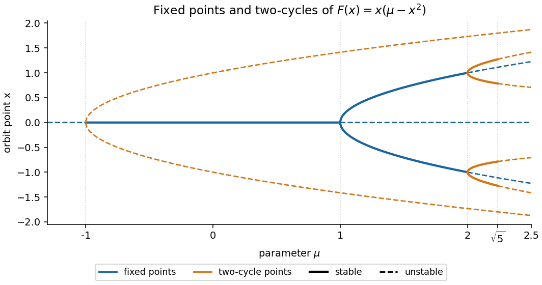
Separate fixed points from roots of . Fixed points are zero, and for . The remaining factors in the given factorization yield first . For these form the symmetric two-cycle because . Its multiplier is , so this cycle is always unstable.
The quartic factor gives for , hence . Positive roots require . At they give the fixed points , not genuine cycles. For , and , giving exactly two additional cycles:There are therefore at most three two-cycles. For either of the latter two, its multiplier isThus they are stable for and unstable for , with a flip at . The nonzero fixed points have multiplier , hence are stable for . Zero is stable for . At there is a supercritical pitchfork; at both nonzero fixed points lose stability to these two-cycles. The symmetric unstable cycle terminates at zero at the subcritical flip . These are the cubic map period-two branches.

Past exam of the mathematics course of the University of Cambridge 2007 ii Paper 4 14E i Solution Created 2026-09-24 Updated 2026-10-14
The fixed-point equation is . Thuswhen the discriminant is nonnegative. At zero the multiplier is , so it is linearly stable for and unstable for . At a nonzero fixed point, eliminate to obtain the branch and its multiplier:The branch is stable precisely when . These formulas specify stability throughout the diagram, including any extra flip points outside the region requested.
If and , the two nonzero branches exist for and have multiplier . Thus is a subcritical pitchfork bifurcation. If , the branch through zero has and ; its stability exchanges with zero at , a transcritical bifurcation. The two nonzero roots meet atwhere . The graph of has nonzero second derivative , proving a saddle-node bifurcation. At zero and , the multiplier is , indicating a period-doubling bifurcation; generically its nondegeneracy coefficient is . If , necessarily here, composition at instead gives . For small, the leading return equation is , producing a two-cycle with leading amplitudes . Its return multiplier is . Thus this special case still has a flip bifurcation, but it is degenerate and subcritical rather than the generic cubic normal form.
For , the fold lies above . Between it and the transcritical point, the branch is stable provided its multiplier remains above , while the other branch is unstable. For , the fold lies below : immediately above it the branch is stable and the branch between and zero is unstable; the branch crossing zero becomes stable for . All these statements are subject to the displayed exact multiplier criterion if the diagram is extended. The sketch uses representative parameter values and stops before additional flips, as stipulated.
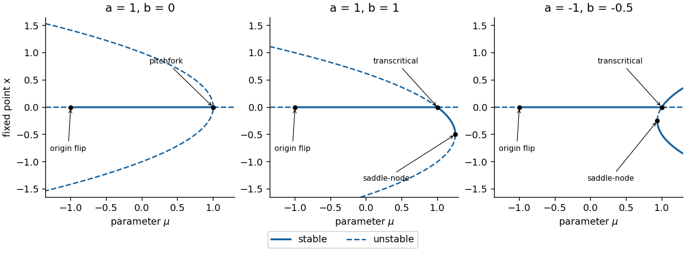
Fixed-point branches and stability for three representative cubic maps, with folds, transcritical or pitchfork crossings, and the origin flip
. Details. 
Past exam of the mathematics course of the University of Cambridge 2007 ii Paper 4 11F ii Solution Created 2026-09-24 Updated 2026-10-14
For odd , pair the terms with denominators and . Since both denominators are coprime to ,has numerator divisible by and denominator not divisible by . Summing these pairs over a common denominator coprime to gives a numerator divisible by . Cancelling common factors cannot remove a factor , since none occurs in the denominator. Therefore the numerator of in lowest terms is divisible by . Equivalently, inversion permutes the nonzero residues and .
Past exam of the mathematics course of the University of Cambridge 2007 ii Paper 4 11F i Solution Created 2026-09-24 Updated 2026-10-14
Compare constant terms in the polynomial identity proved above. The constant term of is , while that of the product is . For odd , this gives . For , the same conclusion holds because . Thus Wilson's theorem follows:
Past exam of the mathematics course of the University of Cambridge 2007 ii Paper 3 8B iii Solution Created 2026-09-24 Updated 2026-10-14
Let . The exponent-sum relation gives . Therefore the assumed boundedness of at infinity makes bounded there, up to a fixed nonzero branch factor. By part (ii), is entire and hence bounded also on compact sets. Liouville theorem makes it a constant , givingIndependence forces : if the Wronskian vanished, uniqueness for the second-order linear equation at an ordinary point would make the two solutions dependent. In fact the differential identity in part (ii) already proves constancy; the boundedness hypothesis supplies the requested Liouville route as well.
Past exam of the mathematics course of the University of Cambridge 2007 ii Paper 3 8B ii Solution Created 2026-09-24 Updated 2026-10-14
For the second-order Fuchsian equation represented by the Papperitz symbol, the coefficient of isThis follows from the sums of local exponents at its two finite regular singular points. Abel's Wronskian identity, obtained by differentiating and using the differential equation, gives . Thus, on every branch domain avoiding zero and one,The normalized expression is locally constant. Its analytic continuation around either singularity is unchanged: the power factors cancel the determinant of the local monodromy, equivalently the integral of around that singularity. It therefore defines a single-valued holomorphic function on the punctured plane, locally constant near both punctures. Those punctures are removable, so the normalized expression extends to an entire function. This argument also covers resonant exponents and avoids assuming two pure power solutions in that case.
Past exam of the mathematics course of the University of Cambridge 2007 ii Paper 3 8B i Solution Created 2026-09-24 Updated 2026-10-14
Let be a local fundamental pair at zero, including a logarithmic Frobenius solution if the exponents are resonant. Any other independent pair on a common branch domain has and with constant coefficients and . Bilinearity and antisymmetry of the Wronskian giveThus changing the independent branches multiplies the principal-pair Wronskian by a nonzero constant, once the branches are continued onto the same domain.
Past exam of the mathematics course of the University of Cambridge 2007 ii Paper 3 38C b Solution Created 2026-09-24 Updated 2026-10-14
With the endpoint values zero, move the new-level differences to the left and keep the old-level differences on the right. Then is tridiagonal with diagonal and off-diagonal entries , while has diagonal and off-diagonal entries . Thus .
Part (a) supplies their common orthonormal eigenbasis. Their eigenvalues are and . For , is invertible, and the step matrix has eigenvaluesSince the eigenbasis is orthonormal, , uniformly in the number of steps and mesh. Hence the method is unconditionally stable for every , which includes all physical positive time steps. For negative , every nonzero modal parameter has modulus larger than one whenever its denominator is nonzero; if a denominator vanishes the step is undefined. Thus the algebraic stable range is exactly . This proof uses simultaneous matrix diagonalization, not Fourier stability analysis.
Past exam of the mathematics course of the University of Cambridge 2007 ii Paper 3 38C a Solution Created 2026-09-24 Updated 2026-10-14
For , extend the proposed vector by . The sine addition identity gives . Thus row-by-row multiplication yieldsThese vectors do not depend on . To prove they form a basis even when eigenvalues of coincide, apply the calculation first to the symmetric matrix with , whose eigenvalues are distinct. Its nonzero eigenvectors are orthogonal and form a basis. Their squared lengths are , so multiplying each by gives a common orthonormal eigenbasis for every matrix in the family.
Past exam of the mathematics course of the University of Cambridge 2007 ii Paper 3 36B ii Solution Created 2026-09-24 Updated 2026-10-14
Independence of and incompressibility give for the secondary velocity . No penetration at the upper and lower walls then forces . The radial momentum equation, retaining the given centrifugal acceleration, is . The transverse pressure gradient is constant in at this order. Integrating twice and absorbing the resulting quadratic coefficient into givesThe odd integration term vanishes because both no-slip conditions are equal. The remaining no-slip and zero-flux conditions areThe second equation is half of . Optionally solving gives and . With the velocity is , so the ratio to the primary velocity is bounded, including its limiting value at the walls, by a constant times . A sufficient parameter ordering isEquivalently the last condition is for . It keeps the secondary circulation weak; the neglected radial return flow and side-wall structure supply closure outside this central wide-channel approximation.
Past exam of the mathematics course of the University of Cambridge 2007 ii Paper 3 36B i Solution Created 2026-09-24 Updated 2026-10-14
The steady axial Navier-Stokes equation for the straight-pipe approximation is . No-slip boundary conditions are . Integrating twice givesIgnoring the radial variation is justified away from the side walls by the given ordering .
Past exam of the mathematics course of the University of Cambridge 2007 ii Paper 3 27J iv Solution Created 2026-09-24 Updated 2026-10-14
European put-call parity givesFor the American call, there are no dividends and the riskless rate is positive, so early exercise sacrifices the benefit of deferring the strike. Directly, at stock 30 its continuation value is , exceeding its exercise value 15; at stock 12 it is , exceeding exercise value zero. At time zero continuation is . Thus , with no optimal early exercise. European parity must not be applied using the American put price .
Past exam of the mathematics course of the University of Cambridge 2007 ii Paper 3 27J iii Solution Created 2026-09-24 Updated 2026-10-14
At the upper time-one node, both exercise and continuation values are zero. At the lower node, immediate exercise gives three while continuation gives , so exercise is strictly better. At time zero immediate exercise gives zero, whereas continuing givesThus continue at time zero and exercise at time one after a down move; at the upper node, exercise or continued holding is immaterial. One initial replicating portfolio for these optimal stopping values is , , costing and producing zero at stock 30 and three at stock 12.
Past exam of the mathematics course of the University of Cambridge 2007 ii Paper 3 27J ii Solution Created 2026-09-24 Updated 2026-10-14
The European put has terminal values . Discounted backward expectation gives value zero at stock 30 and at stock 12. ThereforeFor replication, denote by the money currently in the bank, which grows to next period. At time zero hold shares and , costing . At stock 30 rebalance to zero shares and zero bank balance. At stock 12 rebalance to , . This costs and gives terminal wealth zero at 16 and five at 10. The initial portfolio produces exactly the two node values, so these rebalancings are self-financing.
Past exam of the mathematics course of the University of Cambridge 2007 ii Paper 3 27J i Solution Created 2026-09-24 Updated 2026-10-14
At each nondegenerate binary node, no arbitrage requires the riskless gross return to lie strictly between the two stock returns. The three intervals are at time zero, at the upper node, and at the lower node. Their intersection givesAt , the upper-branch risk-neutral probabilities are . They are initially, after the up move, and after the down move. All are strictly between zero and one, so the martingale measure is equivalent and unique. The four terminal probabilities in the PDF's order are .
Past exam of the mathematics course of the University of Cambridge 2007 ii Paper 3 26I ii Solution Created 2026-09-24 Updated 2026-10-14
Write , with independent of the prior . Then , soCompleting the square in the joint density gives . Thus the Bayes rule is , with Bayes risk . The rule has integrated risk one for every , so its excess Bayes risk is as . The priors remain proper at every positive . Therefore is extended Bayes, without treating the limiting improper flat prior as a proper Bayes prior.
Past exam of the mathematics course of the University of Cambridge 2007 ii Paper 3 26I i Solution Created 2026-09-24 Updated 2026-10-14
For a prior and loss , the Bayes risk of a rule is . A Bayes decision rule minimizes this integrated risk. An Extended Bayes rule is a rule whose excess over the optimal Bayes risk can be made arbitrarily small by a suitable proper prior: for every some has , with finite risks.
Condition on the observation and use iterated expectation. A rule is Bayes precisely when it chooses a minimizer of the posterior expected loss almost surely, up to the usual measurability requirement. Under squared Euclidean loss, with a finite posterior second moment, write . The identityshows that the Bayes rule is the posterior mean.
Past exam of the mathematics course of the University of Cambridge 2007 ii Paper 3 25J e Solution Created 2026-09-24 Updated 2026-10-14
Past exam of the mathematics course of the University of Cambridge 2007 ii Paper 3 25J d Solution Created 2026-09-24 Updated 2026-10-14
Past exam of the mathematics course of the University of Cambridge 2007 ii Paper 3 25J c Solution Created 2026-09-24 Updated 2026-10-14
If , then . Induction gives . Summing the matrix-exponential series yieldsThus deviations of total mass zero decay with the single rate .
There are unlisted articles, also show them or only show them.