
2-adic valuation Created 2026-09-24 Updated 2026-09-28
Orthonormal coframe in spacetime Created 2026-09-24 Updated 2026-10-14
Rotational invariance of a central-potential Hamiltonian Created 2026-09-24 Updated 2026-09-24
Angular momentum ladder variable Created 2026-09-24 Updated 2026-09-29
Squared orbital angular momentum in position and momentum operators Created 2026-09-24 Updated 2026-09-24
Operator ordering gives
Angular momentum ladder operator Created 2026-09-24 Updated 2026-10-03
The operators satisfyThey therefore change the magnetic quantum number by while preserving the total angular-momentum quantum number .
Orbital angular momentum commutation relations Created 2026-09-24 Updated 2026-09-24
Rotation commutators for orbital angular momentum Created 2026-09-24 Updated 2026-09-29
Fixed-tension partition function of a one-dimensional chain Created 2026-09-24 Updated 2026-09-24
Harmonic coordinate Created 2026-09-24 Updated 2026-10-06
A harmonic coordinate satisfies for a Riemannian metric, or for a Lorentzian metric. Equivalently or . This common coordinate condition applies in both Riemannian geometry and general relativity.
3+1 decomposition of spacetime Created 2026-09-24 Updated 2026-10-14
Quadrature rule Created 2026-09-24 Updated 2026-10-14
A quadrature rule approximates an integral by a finite weighted sum of sampled function values:The quadrature nodes specify where to sample, and the quadrature weights specify how much each sample contributes. The density specifies the target integral, whereas the discrete quadrature weights belong to the approximation. Ordinary numerical integration has . Gaussian quadrature and the midpoint quadrature rule choose interior quadrature nodes; the trapezoidal rule includes endpoints.[ref]
For ordinary numerical integration, exactness on the constant function requires ; exactness on additionally requires . These two checks make the quadrature rule exact for every affine function. For example, both the midpoint quadrature rule and trapezoidal rule give for . Testing progressively higher polynomial degrees defines the degree of precision of a quadrature rule. Exactness describes a class of integrands, rather than promising exact results for every function.
Composite midpoint quadrature rules and composite trapezoidal rules apply a simple quadrature rule on every panel of a partition of an interval. This buys accuracy by shrinking the panels while keeping the elementary formula fixed. For continuous functions sampled exactly, their quadrature errors tend to zero as the largest panel width tends to zero. The familiar second-order bounds require stronger assumptions about derivatives. The signed approximation error used here is ; some sources define quadrature error with the opposite sign, so the convention must accompany any formula.
Orthogonal polynomial Created 2026-09-24 Updated 2026-10-18
An orthogonal polynomial family chooses polynomials that do not overlap under a specified inner product. For real polynomials on an interval , use the weighted inner productAssume , the weight is measurable and positive almost everywhere, and its absolute moments are finite for every integer . These conditions make the integrals finite and give every nonzero polynomial positive squared norm. A sequence is an orthogonal polynomial family when has real coefficients and polynomial degree exactly , and for .[ref]
18 Orthogonal Polynomials. NIST Digital Library of Mathematical Functions; Koornwinder, Wong, Koekoek, Swarttouw and Reinhardt, NIST DLMF Chapter 18, §18.2(i), equations 18.2.1 and 18.2.1_5: interval orthogonality and finite absolute moments
Here and is the Kronecker delta. Orthogonality does not require : an orthonormal set is obtained only after replacing by . Multiplying each member by any nonzero real constant preserves orthogonality, but changes its norm and the corresponding expansion coefficient. The monic orthogonal polynomial convention instead fixes each leading coefficient to one.
The first four Legendre polynomials, named for Adrien-Marie Legendre, use on and the normalization :Their orthogonality and squared norms areThus their Gram matrix has a positive diagonal and zero entries elsewhere, although their function graphs cross and overlap on the page. Orthogonality measures an integral of products, rather than separation of function graphs.[ref]
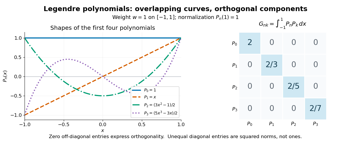
The first four Legendre polynomials and their exact integral Gram matrix: orthogonal, with unequal squared norms
. Details. 
For these four polynomials, a short verification expands each product and uses and . For example, and . The same calculation gives the diagonal entries . More generally, apply the Gram-Schmidt process to the monomial basis : at step , subtract projections onto the earlier polynomials. The result retains its leading term, has degree , and has positive norm, proving existence without a differential equation. Different degrees also give linear independence, so form a basis of the polynomials of degree at most .
This basis turns least-squares solutions for functions into independent scalar calculations, as the decoupled coefficients of orthogonal polynomial projections show. In a spectral method, increasing the degree enlarges the approximation space while keeping earlier projection coefficients fixed. Weighted integrals also connect the same orthogonal polynomials to Gaussian quadrature: its nodes are polynomial roots of a member of the family. The projection problem minimizes an integrated squared error; Gaussian quadrature uses the family to choose evaluation points for an integral.
Linear stability domain Created 2026-09-24 Updated 2026-10-03
For a one-step method applied to , write . Its linear stability domain isForward Euler has , while backward Euler has and is A-stable.
Numerical linear algebra Created 2026-09-24 Updated 2026-10-14
Stability function Created 2026-09-24 Updated 2026-09-24
Sparse optimization Created 2026-09-24 Updated 2026-09-24
Simplex algorithm Created 2026-09-24 Updated 2026-10-31
Runge-Kutta method Created 2026-09-24 Updated 2026-10-31
A Runge-Kutta method advances an initial value problem , , by sampling its vector field at several trial states within one time step. These samples are Runge-Kutta stages; a weighted combination of their slopes produces the next state. The construction improves on the single tangent line used by the Euler method while requiring evaluations of , rather than explicit higher derivatives of the solution. It applies to scalar equations and systems of ordinary differential equations alike. The coefficient choices distinguish methods such as Heun's method, the classical fourth-order Runge-Kutta method and implicit Runge-Kutta methods.
For stages, write for the stage matrix, for relative time nodes and for output weights. A time step of length computesHere is a slope, with units of state per time; is a state increment. Another common convention writes , so its stage states are and its output is . These are equivalent conventions: including both inside and again in the output would count the time step twice. The textbook formulation uses the increment convention.[ref]
6.4 Runge-Kutta methods. Fundamentals of Numerical Computation, §6.4.3, equations 6.4.10–6.4.11: multistage recipe and tableau
Usually the Butcher tableau obeys , called internal consistency. Stage then combines slopes over an effective time . The second-order conditions with independent Runge-Kutta abscissae explain what changes when time nodes are specified independently. A Runge-Kutta stage is generally an auxiliary approximation, not a separate accepted solution value at its node. Several stages can even have the same time node but different state arguments, as in the classical fourth-order Runge-Kutta method.
The useful idea is to approximate the integral without knowing the intermediate exact trajectory. Trial states provide places to sample , and Butcher order conditions make the resulting combination agree with the exact Taylor expansion. More stages alone do not guarantee a higher order of a numerical method: their coefficients must satisfy the appropriate conditions. Embedded Runge-Kutta pairs reuse these same samples for a second output and a practical local error estimator.
Fourier spectral method for variable-coefficient advection Created 2026-09-24 Updated 2026-09-24
There are unlisted articles, also show them or only show them.