
Multiplicative inverse Created 2026-09-24 Updated 2026-10-18
Isomorphism Created 2026-09-24 Updated 2026-10-14
An isomorphism is a morphism with a two-sided inverse that is also a morphism. Two objects are isomorphic when such a map exists between them. For groups, rings, and vector spaces, a bijective structure-preserving map has a structure-preserving inverse; in other settings the inverse condition needs separate attention, as for a homeomorphism between topological spaces.
For example, is a group isomorphism from the additive integers to the additive even integers. It is bijective onto that target, satisfies , and has inverse . The two groups have the same addition pattern even though they are different sets. It is not a ring isomorphism for their inherited multiplications, since while .
Endomorphism Created 2026-09-24 Updated 2026-10-14
An endomorphism is a morphism : its source and target are the same object, with the same specified structure. For a group it is an operation-preserving group homomorphism back into that group; for a vector space it is a linear endomorphism; for a ring it is a ring endomorphism. A self-map must satisfy the chosen compatibility conditions to qualify. The notation records the category in which these conditions are imposed. See Riehl, Category Theory in Context, Definition 1.1.10 and the following paragraph.
An endomorphism can lose information or miss part of its target. On the additive integers, preserves addition and is injective, but is not surjective: no integer maps to . On the vector space over the real numbers, the linear endomorphism loses the second coordinate, so it is neither injective nor surjective. Neither is an automorphism. The same doubling rule becomes a group isomorphism when its target is the additive even integers, as explained under isomorphism.
The finite cyclic group offers a small example of information loss that can be drawn completely. With addition in modular arithmetic, the endomorphism sends the inputs to . Its image of a group homomorphism is and its kernel of a group homomorphism is . Each reached output has two inputs; the other three outputs are missed.
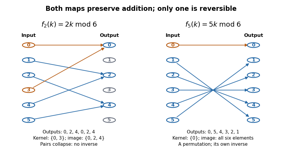
For an endomorphism of a group or ring with a finite underlying set, injectivity is equivalent to surjectivity by counting; either condition makes it an automorphism. The additive integers example shows why the finiteness assumption matters. A linear endomorphism of a finite-dimensional vector space also has equivalent injectivity and surjectivity, this time by the rank-nullity theorem even when its underlying set is infinite.
Self-maps can be iterated without changing the object: , , and so on. Composition in a category and the identity morphism make the endomorphisms of a fixed object in a locally small category into a monoid. This packages repeated compatible operations, including irreversible ones, into a single structure.
The general language has a documented historical milestone in the 1945 paper of Samuel Eilenberg and Saunders Mac Lane. They defined categories of objects and compatible maps, and distinguished maps admitting inverses within that category. Their examples included groups, vector spaces, and topological spaces. This gave a common framework for compatible self-maps and their invertible cases. See Eilenberg and Mac Lane, General Theory of Natural Equivalences, pp. 234 and 237–239.
Importance sampling Created 2026-09-24 Updated 2026-09-24
To estimate , sample independently from a reference density whose support covers that of , and useThe summands have expectation , and the strong law of large numbers gives almost-sure convergence under integrability.
Rejection sampling Created 2026-09-24 Updated 2026-10-14
Suppose is a target probability density and is a proposal density with . Draw and an independent , and accept whenThe accepted value has density , the acceptance probability is , and the expected number of proposals is .
Canonical commutation relation Created 2026-09-24 Updated 2026-09-28
Angular momentum Created 2026-09-24 Updated 2026-10-14
Angular momentum measures how a point mass's momentum passes around a chosen origin. Motion straight toward or away from that origin contributes zero; transverse momentum contributes more when it passes farther away. The picture shows the sign convention before the calculation.
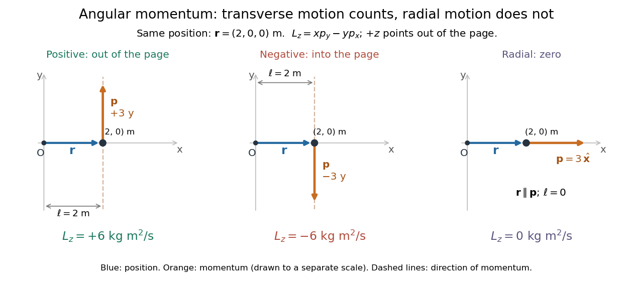
Positive, negative and zero angular momentum about the same origin
. Details. Fix an origin and nonrotating axes in an inertial frame. For a nonrelativistic point mass of constant mass , let be its position from and its mechanical momentum in that same reference frame. Its angular momentum is the cross productHere , , and is the angle between them. The right-hand rule gives the direction: curl from toward , and the thumb points along . Thus angular momentum is an axial vector, perpendicular to both position and momentum. Its International System of Units unit is . A point mass need not follow a circle to have angular momentum.[ref]
With rightward, upward, and out of the page, the cross product gives . TakeThen . Reversing the momentum makes ; radial momentum gives . The factor is the lever arm to the line through the particle parallel to its momentum.
For motion in the plane, plane polar coordinates give , with . ConsequentlyThe signed angular velocity is positive counterclockwise viewed from toward the plane, with measured in radians. Radial velocity does not enter the cross product. Under conservation of angular momentum, this relation predicts faster angular motion at smaller and constant areal velocity for consistently oriented swept area. That is the geometric content of Kepler's second law.
For several point masses, add their angular momenta about the same origin: . The origin matters: angular momentum under an origin shift explains why the same moving particle can have different values about two fixed points. The central axis of a momentum system and angular momentum decomposition about the centre of mass make this dependence useful.
Rocket equation Created 2026-09-24 Updated 2026-10-14
The ideal rocket equation gives the change in signed velocity produced by ejecting rocket propellant. Assume one-dimensional Newtonian mechanics in an inertial frame, no external force, and a fixed positive rocket exhaust speed directed rearward relative to the instantaneous rocket. The rocket's instantaneous mass includes its remaining rocket propellant; burning it gives . For initial and final masses ,Here is the natural logarithm, and its argument is the rocket mass ratio. This is the constant-rocket exhaust speed, zero-pressure-correction version of the ideal rocket equation. [ref]
For a toy rocket with , and rocket dry mass after all rocket propellant is spent, the rocket mass ratio is andBurning from to gains . Burning from to gains exactly the same velocity increment, using only of rocket propellant instead of . Both burns halve the remaining mass. The second burn accelerates a lighter rocket; equal fractional mass losses give equal velocity gains.
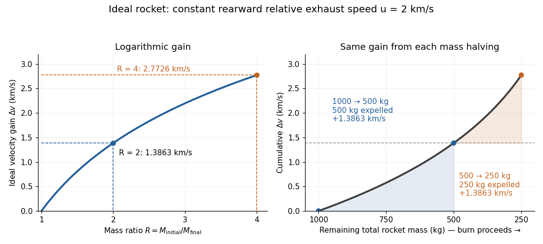


The natural logarithm makes the rocket equation both useful and revealing: multiplying successive rocket mass ratios adds their velocity gains. Conversely, the required rocket mass ratio is the exponential function . Each extra of ideal velocity gain doubles the required initial mass for fixed final mass. This explains why a larger rocket exhaust speed is valuable and why carrying ever more rocket propellant has diminishing returns. Changing the burn duration alone does not change this ideal endpoint result.
For a short proof outline, follow the rocket together with a tiny parcel about to be expelled. Before ejection, their total momentum is . After ejection, the remaining rocket has mass and velocity , while the parcel has positive mass and, to first order, inertial velocity . Momentum conservation givesDiscarding the second-order product gives ; taking the integral gives . Evaluating the integral yields the natural logarithm above. This is a variable-mass system calculation: the rocket alone is not a closed system, and its momentum changes as the expelled material carries away momentum. The fixed collection consisting of the rocket and all its expelled material has conserved total momentum when external forces vanish.
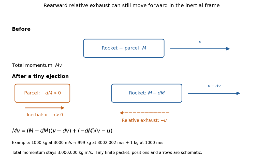
Momentum balance for a tiny expelled parcel: rearward relative exhaust can still move forward in the inertial frame
. Details. 
Fixed rocket exhaust speed means fixed relative speed at release, not fixed inertial velocity. As the rocket's velocity changes, newly emitted material has changing inertial velocity ; previously released parcels coast at their own release velocities in this ideal model. If , the exhaust even moves forward in the inertial frame, although it is emitted rearward relative to the rocket. No surrounding medium is needed for this exchange of momentum.
Real flight adds gravity, drag force and possibly a pressure correction to rocket thrust. A varying rocket thrust due solely to a changing mass loss rate still gives the same ideal rocket equation if is constant; it changes the acceleration and burn duration. A changing rocket exhaust speed instead requires , and external forces require their own contribution to the velocity change. The existing constant mass-loss propulsion with quadratic drag and constant-burn rocket with ground friction illustrate such additional forces; the forward-exhaust rocket equation reverses the ejection direction and therefore the sign of the recoil.
Residue class Created 2026-09-24 Updated 2026-10-14
For a positive integer modulus , the residue class of an integer is the equivalence classIt contains all integers in the same position of the repeating cycle. For example,The residue class is this whole infinite collection; its canonical representative is the least nonnegative residue. Euclidean division gives exactly one such representative in , so there are exactly residue classes. When , there is just one, .
Define addition and multiplication of residue classes byThese definitions must give the same answer whichever integers represent the classes. If and modulo , thenBoth differences are divisible by , proving that the operations are well-defined. For example, and , since . Replacing nine by gives the same answers with smaller intermediate integers.
With these operations the residue classes form the finite commutative ring , a quotient ring. It need not be a field: although neither factor is the zero class. These zero divisors explain why division requires a unit modulo n. Reducing after each multiplication is especially useful in modular exponentiation, where the unreduced powers can become enormous.
Strongly minimal theory Created 2026-09-24 Updated 2026-10-14
A complete theory is strongly minimal when every definable one-variable subset of every model is finite or cofinite.
Elementary extension Created 2026-09-24 Updated 2026-10-14
An elementary extension is an extension preserving all first-order truth with parameters, hence giving elementary equivalence. An extension is elementary when every formula with parameters from has the same truth value in both structures.
Ultraproduct Created 2026-09-24 Updated 2026-09-24
An ultraproduct identifies two sequences when they agree on a set belonging to an ultrafilter and interprets symbols coordinatewise.
Quantifier elimination Created 2026-09-24 Updated 2026-09-24
Complete theory Created 2026-09-24 Updated 2026-10-14
A consistent first-order theory is complete when it decides every sentence in its language.
Minkowski metric Created 2026-09-24 Updated 2026-10-14
With the mostly-plus metric signature and coordinates , the Minkowski metric is the nondegenerate bilinear formIt is a symmetric bilinear form, but not a positive-definite bilinear form. For example, is nonzero yet , making it a null vector. This does not make the Minkowski metric degenerate: some other vectors have nonzero pairing with .
Applied to infinitesimal displacements, the Minkowski metric givesFor a timelike curve, a clock records . For a null curve, . For spacelike separation, the positive Minkowski interval measures a different kind of separation. A Lorentz transformation preserves this form, expressed in matrix notation by , although it need not preserve ordinary Euclidean distance in the four-component coordinate list.
Inverse metric Created 2026-09-24 Updated 2026-10-03
Source-free Maxwell equations in a linear medium Created 2026-09-24 Updated 2026-09-24
Covariant Maxwell equation with the minus-plus-plus-plus metric Created 2026-09-24 Updated 2026-09-24
With metric signature , , and , the field tensor satisfiesIts components are and , so these tensor equations reproduce all four Maxwell equations.
Charge conservation from Maxwell equations Created 2026-09-24 Updated 2026-09-24
Taking the divergence of the Ampère-Maxwell equation and using Gauss's law givesHence the charge in a fixed volume changes only through current crossing its boundary.
Gauss's law Created 2026-09-24 Updated 2026-10-14
Gauss's law relates the electric field on a closed surface to the net electric charge inside it. In SI units, with outward unit normal ,Here describes a volume charge density, and is the vacuum permittivity; for ideal point or surface charges, use the enclosed electric charge directly rather than an ordinary volume-density integral. The left side is electric flux: the surface integral of the outward normal component of the electric field. Field directed outward contributes positively; field directed inward contributes negatively. The equality uses net signed electric charge, so positive and negative enclosed charges can cancel. The Gaussian surface is an imagined accounting boundary, not necessarily a material object. See OpenStax, explaining Gauss's law.
Where the electric field and charge density are smooth, the local statement is . The divergence theorem connects this divergence to the surface integral. This is the satisfying connection between local sources and global accounting: a surface can register how much net electric charge it encloses without revealing where that charge is located within it. A point charge requires care with the singular field at its position; the integral formulation remains useful with a boundary that avoids the charge.
The law fixes total electric flux, rather than every value of the electric field. In an uncharged region, a uniform electric field crosses a cube of side . Its left and right faces contribute and ; the other four faces contribute zero. Thus the net electric flux is zero while the electric field is nonzero everywhere. Charges outside a Gaussian surface can change the field on it without changing its net electric flux. Conversely, fields cannot generally be reconstructed from enclosed electric charge alone. Electrostatics also requires the electric field to be the negative gradient of an electric potential, with appropriate boundary information. This distinction is emphasized in Feynman lectures II.5, application of Gauss' law.
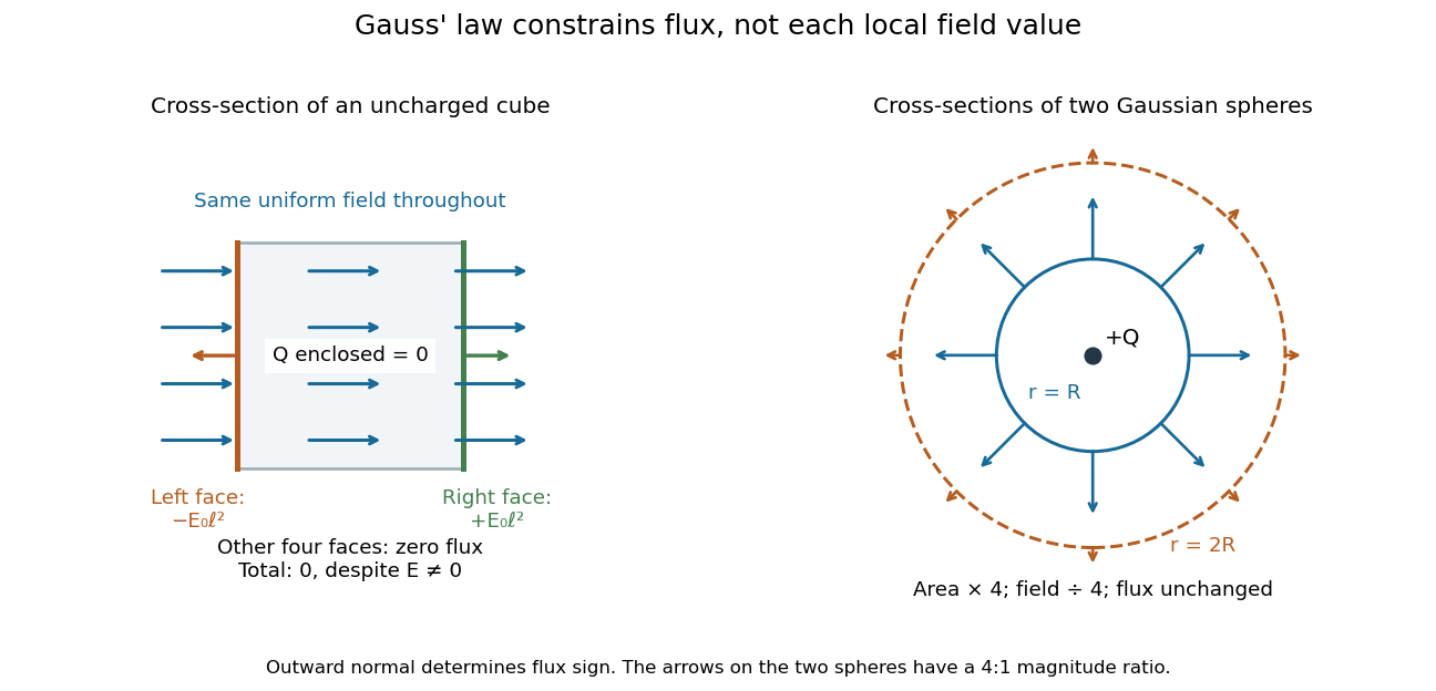
Zero net flux can coexist with a nonzero uniform field, and equal enclosed charge can give different field magnitudes on different spheres
. Details. 
Spherical symmetry supplies the extra information needed for a particularly simple calculation. An isolated spherically symmetric charge distribution in vacuum produces a radial electric field, constant in magnitude on each concentric sphere. Its electric flux is therefore , givingOutside the distribution, doubling quadruples the surface area and divides the radial electric field by four, while the electric flux stays . The inverse-square dependence is an area-dilution result. The electric field of a uniformly charged ball and electric field of a uniformly charged spherical shell show that the same total charge can give different interior fields. These symmetry arguments and their limits are developed in OpenStax, applying Gauss's law.
There are unlisted articles, also show them or only show them.