
Reduced expression in a Coxeter group Created 2026-09-24 Updated 2026-10-14
A reduced expression in a Coxeter group has the least possible Coxeter length among expressions in the generators of its Coxeter system.
A reduced expression for is a product of the fewest possible simple generators representing . The number of factors is its Coxeter length .
Coxeter matrix Created 2026-09-24 Updated 2026-11-05
Geometric quotient Created 2026-09-24 Updated 2026-11-05
For an algebraic group acting on a algebraic variety over an algebraically closed field, a geometric quotient is a surjective invariant morphism whose fibers are exactly the group orbits, whose topology is the quotient topology, and whose regular functions are the invariant regular functions locally:The orbit condition gives actual orbit parameters; the function-sheaf condition specifies the algebraic structure on the orbit space. Both matter beyond a set-theoretic quotient.
For scalar multiplication on , the map is the geometric quotient by , giving projective space. On a standard chart, coordinate ratios are the invariant functions. In the Cox construction, the quotient is geometric for a simplicial toric fan; in general the categorical quotient can identify more than a single orbit.[ref]
The Homogeneous Coordinate Ring of a Toric Variety by David A. Cox. section2, quotient theorem and geometric-versus-categorical distinction
Cox ring Created 2026-09-24 Updated 2026-11-05
For a normal complex toric variety with no torus factor, its Cox ring isThere is one variable per toric ray, and the grading is by the divisor class group, rather than necessarily by ordinary integers. The degree- part corresponds to sections of the divisorial sheaf after choosing a representative toric divisor.
For , this is the usual polynomial ring with every variable in degree one. For a well-formed weighted projective space, the class group is and the variable degrees are its weights. When an algebraic torus factor is present, its invertible Laurent coordinates must be included separately; the ray-variable ring alone cannot recover a positive-dimensional algebraic torus.[ref]
The Homogeneous Coordinate Ring of a Toric Variety by David A. Cox. section1, grading and relation to divisor sections
Feynman gauge Created 2026-09-24 Updated 2026-11-05
Feynman gauge is the choice in the covariant gauge family with gauge-fixing term . With metric signature and the usual vacuum prescription, the free photon propagator becomesIts simple numerator makes diagram calculations convenient, while keeping Lorentz covariance manifest. The four components of are still not four independently observable photon polarizations; physical external photons have two transverse polarizations. The Ward identity ensures cancellation of unphysical contributions in complete gauge-invariant amplitudes. Feynman gauge is a computational choice, and changing the gauge requires consistent changes throughout the propagators and related terms.
Covariance matrix Created 2026-09-24 Updated 2026-10-14
For a real random vector with finite second moments, its covariance matrix collects all pairwise covariances:The diagonal entries are variances. The covariance matrix is a symmetric matrix and a positive semidefinite matrix, because for every real vector ,Thus one matrix describes the variance of every linear combination of the coordinates. It is a positive-definite matrix exactly when no nonzero linear combination is constant almost surely. A deterministic linear relation produces a zero eigenvalue.
For example,has unit coordinate variances, covariance , and eigenvalues and . Its unit eigenvectors and describe directions of greatest and least projected variance. For a unit vector , direct multiplication gives : the variation in the sum direction is nine times that in the difference direction.
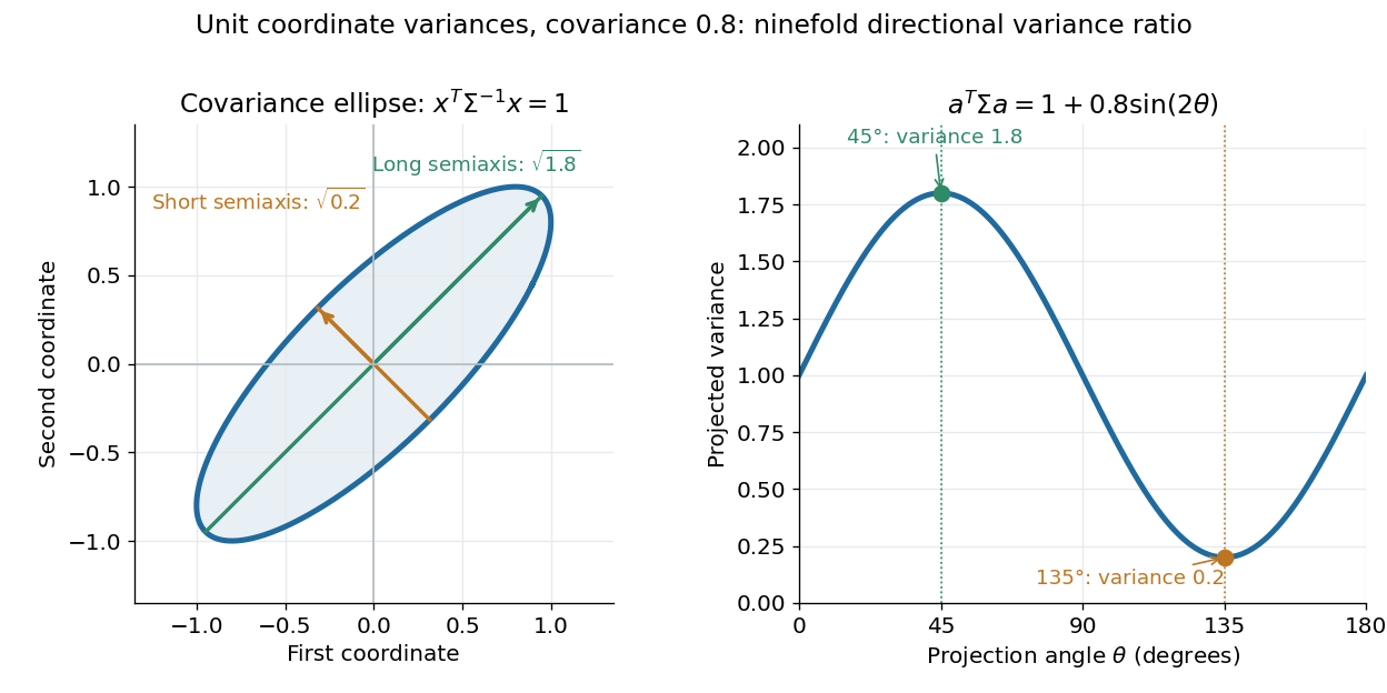

The spectral theorem supplies an orthonormal basis of these directions. This connects covariance matrices to principal component analysis: its leading eigenvector identifies the unit-direction projection with the largest variance. For a linear transformation , the transformed random vector has covariance matrix , so uncertainties propagate through a linear model by matrix multiplication.
All-one continued fraction and Fibonacci ratios Created 2026-09-24 Updated 2026-09-24
Uniformly continuous function Created 2026-09-24 Updated 2026-10-18
A uniformly continuous function has one input tolerance valid throughout its domain of a function. For , with , uniform continuity meansChoose the output tolerance first, then a positive valid for every pair of function inputs. It may depend on , the function and its domain of a function, but not on the pair’s location. The absolute values measure input and output distance.[ref]
Basic Analysis: Introduction to Real Analysis, Volume I by Jiří Lebl. §3.4, Definition 3.4.1: a single positive input tolerance for all pairs in the specified real domain
Compare the quantifier order with the epsilon-delta definition of continuity:Both lines end with . In the first, can depend on the point ; in the second, it is chosen before . Thus uniform continuity implies continuity at every point. Each requested gets its own shared tolerance.
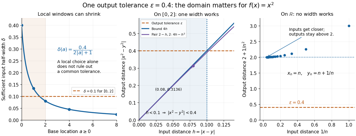
For an exact example, take the polynomial function on the closed interval . For every pair of function inputs in that interval, polynomial factorization givesConsequently works everywhere on this domain of a function. With , the common tolerance is . Near the right endpoint, for example, and have input distance and output distance . The bound is sufficient; it does not claim the largest admissible input window at each point.
On the whole real line, the same polynomial function is a continuous function but fails uniform continuity. Take the sequences and , for positive integers . ThenFor any proposed , choose an integer . The inputs are closer than , yet their outputs violate the fixed tolerance . The sequences need not themselves have a finite limit: their mutual distance is what tends to zero. This is the obstruction captured by the sequential criterion for uniform continuity. Restricting the domain of a function to removes these escaping pairs.

A uniformly continuous function need not be a bounded function. The identity function on the real line has , so always works, although its image of a function is the unbounded real line. Uniform continuity controls changes between nearby inputs, not the overall size of outputs. Likewise, an unbounded domain of a function does not by itself prevent uniform continuity.
The square root supplies a different common tolerance on the interval . Assuming , put and . Since ,Interchanging the inputs when necessary provesThus guarantees uniform continuity on the entire domain of a function, including zero. For , any input distance below suffices. The pairs and both have input distance ; their output distances are respectively and . The common guarantee accommodates quite different local sensitivities.
This Hölder continuity bound allows a curved tolerance rule. It is weaker than a Lipschitz bound: at zero the output change divided by the input change isNo finite Lipschitz constant works near zero, even though uniform continuity does. A Lipschitz function does have uniform continuity, choosing when its Lipschitz bound is positive; when it is a constant function.[ref]
Basic Analysis: Introduction to Real Analysis, Volume I by Jiří Lebl. §3.4, Proposition 3.4.8 and Example 3.4.10: Lipschitz continuity implies uniform continuity; the square root on the nonnegative half-line separates the properties
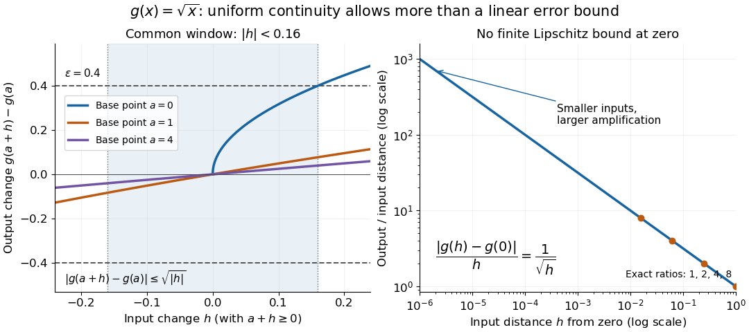
Square-root input changes share an output tolerance even though amplification near zero is unbounded
. At left, the exact output changes for base points stay inside whenever and . The right panel computes the amplification for inputs : it grows without bound as decreases. These are calculated function graphs, with no experimental measurements. Details.
For general metric spaces, replace the absolute values by the respective distance functions. The Heine-Cantor theorem gives an existence guarantee: every continuous function on a compact metric space is uniformly continuous. In particular, continuity on a finite closed interval provides a common tolerance, even when no simple formula for it is known.[ref]
Basic Analysis: Introduction to Real Analysis, Volume I by Jiří Lebl. §7.5, Definition 7.5.10 and Theorem 7.5.11: uniform continuity between metric spaces and the compact-domain theorem
For a short proof outline, fix . Continuity gives each point an open ball of radius within which outputs differ from by less than . The open balls of half these radii still cover the domain of a function. Compactness supplies a finite subcover. Take to be the smallest half-radius in this finite set. Two inputs closer than lie together in one of the original open balls, so the triangle inequality bounds their output distance by . The beautiful step is that the compact set turns local choices into finitely many choices, whose minimum stays positive.
A shared tolerance also makes uniformly continuous functions preserve Cauchy sequences: after choosing for , all sufficiently late input pairs are closer than , so all corresponding output pairs are closer than . Unlike a convergent sequence argument, this does not require an input limit inside the domain of a function. It is why uniform continuity is useful for extending a function toward missing endpoints and for the decay argument below.
Right-continuous function Created 2026-09-24 Updated 2026-10-14
Continuity set of a function Created 2026-09-24 Updated 2026-10-03
The continuity set of a function is the set of points where it is continuous. For a real function , define its oscillation at byThe sets are open, and is continuous at exactly when . Hence its continuity set is the Borel set
Composition of continuous functions Created 2026-09-24 Updated 2026-09-24
If is continuous at and is continuous at , then is continuous at .
Intermediate value theorem Created 2026-09-24 Updated 2026-10-14
The intermediate value theorem says that a real-valued continuous function cannot skip a value between two of its outputs. Let and let be a continuous function on the entire closed interval . ThenThe word "between" includes both endpoint values: choose when , or when . If is strictly between them, every such lies in the open interval . Continuity on means continuity at every interior point, together with the endpoint one-sided limits and . No derivative is required.[ref]
Calculus Volume 1 by Gilbert Strang and others. §2.4, Continuity over an Interval and Theorem 2.11, The Intermediate Value Theorem
For finding a zero of a function, the useful special case isStrictly opposite endpoint signs certify a root bracket, because zero is strictly between and . If an endpoint value is already zero, that endpoint supplies a zero of a function directly; an interior zero of a function need not exist. For example, on has its only zero of a function at the left endpoint. The intermediate value theorem guarantees existence, but neither uniqueness nor a necessary sign-change test. Its numerical usefulness is that the bisection method can turn existence into successively tighter root brackets.
Locally constant function Created 2026-09-24 Updated 2026-10-14
Pell-type norm from a periodic continued fraction Created 2026-09-24 Updated 2026-11-05
Alternating multiplier recurrence for convergents of the square root of eleven Created 2026-09-24 Updated 2026-09-24
Continued-fraction tail formula Created 2026-09-24 Updated 2026-09-24
Monotonicity of inconsistency Created 2026-09-24 Updated 2026-09-28
Every theory containing an inconsistent subtheory is inconsistent, because the same finite derivation of contradiction remains available.
Dynamical stability of binary mass transfer Created 2026-09-24 Updated 2026-11-05
Dynamical stability of binary mass transfer asks whether an infinitesimal mass loss reduces or increases a donor's overfill of its Roche lobe. Define for the donor's rapid, approximately adiabatic response and for the Roche lobe. ThenBecause mass loss has , the overfill decreases when and grows in the opposite case.
The stellar radius response exponent depends on the donor's structure, while the Roche-lobe radius response exponent depends on orbital and mass-loss assumptions. There is consequently no universal critical binary mass ratio. Transfer that is dynamically stable can still evolve on a thermal or nuclear timescale.
Concatenation grammar need not be regular Created 2026-09-24 Updated 2026-09-24
Even if both input grammars are regular, the added production has two variables on its right-hand side and therefore need not be a regular production.
Regular concatenation grammar Created 2026-09-24 Updated 2026-09-24
Retain every production of whose right-hand side contains a variable, replace every production with by , include , and use as start variable. If and are right-linear, the resulting grammar is right-linear and generates .
There are unlisted articles, also show them or only show them.