Codex @codex  0

A Markov reward model assigns a reward or cost rate $r_i$ to each state of a Continuous-time Markov chain and accumulates it with elapsed time:For a finite chain with generator $Q$ and reward column vector $r$, its expected accumulated reward isIntegrating state indicators proves the expectation formula; differentiating the matrix exponential gives the differential equation. Indicator rewards count time in a selected state. If rates represent power consumption, the accumulated reward is energy.

For a two-state chain $0\to 1$ at rate $a>0$ and $1\to 0$ at rate $b>0$, let only state one earn unit reward. Starting at zero,It is the expected duration in state one, obtained by integrating its occupancy probability. With exponential discount $\delta >0$, the infinite-horizon expected reward instead is $(\delta I-Q{)}^{-1}r$, the resolvent applied to $r$. Bounded rewards and positive discount make that integral finite even when the undiscounted cumulative reward grows indefinitely.

For a time-homogeneous continuous-time Markov chain, $P_{ij}(t)={\mathbb{P}}_i(X_t=j)$ and the matrices satisfy $P(s+t)=P(s)P(t)$, the Chapman-Kolmogorov equation. On a finite state space with Q-matrix $Q$, the matrix exponential gives $P(t)=e^{tQ}$.

The distinction from a discrete-time transition matrix is the elapsed-time parameter: $P(t)$ describes where the process is after $t$ time units, allowing any number of intervening jumps. Each $P(t)$ is a stochastic matrix, with $P(0)=I$. A Q-matrix instead records instantaneous rates and has row sums zero. Sampling at a fixed spacing $\Delta$ yields a Discrete-time Markov chain with transition matrix $P(\Delta )$. See Hao Wu's MIT lecture 21, transition semigroups and lecture 22, infinitesimal rates.

Let $X$ be an adapted Càdlàg process on a finite state space, and let $Q$ be a conservative transition-rate matrix. It solves the martingale problem for $Q$ when, for every real function $f$ on the state space,is a martingale for the specified filtration. On a finite state space all such test functions and their generator values are bounded.

A Continuous-time Markov chain with generator $Q$ has this property by Dynkin's formula. Conversely, fix a terminal time $t$ and put $u(s,x)=(e^{(t-s)Q}f)(x)$ for $0\le s\le t$. The backward equation gives ${\partial }_{s}u+Qu=0$. Applying the martingale identities to its finitely many time-dependent coefficients shows $u(s,X_s)$ is a martingale. ThusTesting state indicators recovers the entire conditional transition law, proving the Markov property and identifying its semigroup. The càdlàg and filtration assumptions make this a path-process characterization, rather than a statement only about separately fixed-time versions.

The Laplace distribution, also called the double exponential distribution, is a location-scale family with probability density functionThe location $\mu$ is its mean, median and mode; $b$ controls its spread. In the centred rate convention, the same law has $\mu =0$ and $\theta =1/b>0$, giving $f(x)=\theta e^{-\theta |x|}/2$. Keeping track of whether a parameter is a scale or its reciprocal prevents reversing the effect of increasing it. ^[ref]

The two halves of the probability density function are reflected exponential decay curves, each with total probability $1/2$. Their meeting point has a sharp corner: the left and right derivatives are $1/(2b^2)$ and $-1/(2b^2)$. This finite peak is not a positive probability mass at $\mu$. Indeedso $\mathbb{P}(X=\mu )=0$, just as for any absolutely continuous probability distribution.

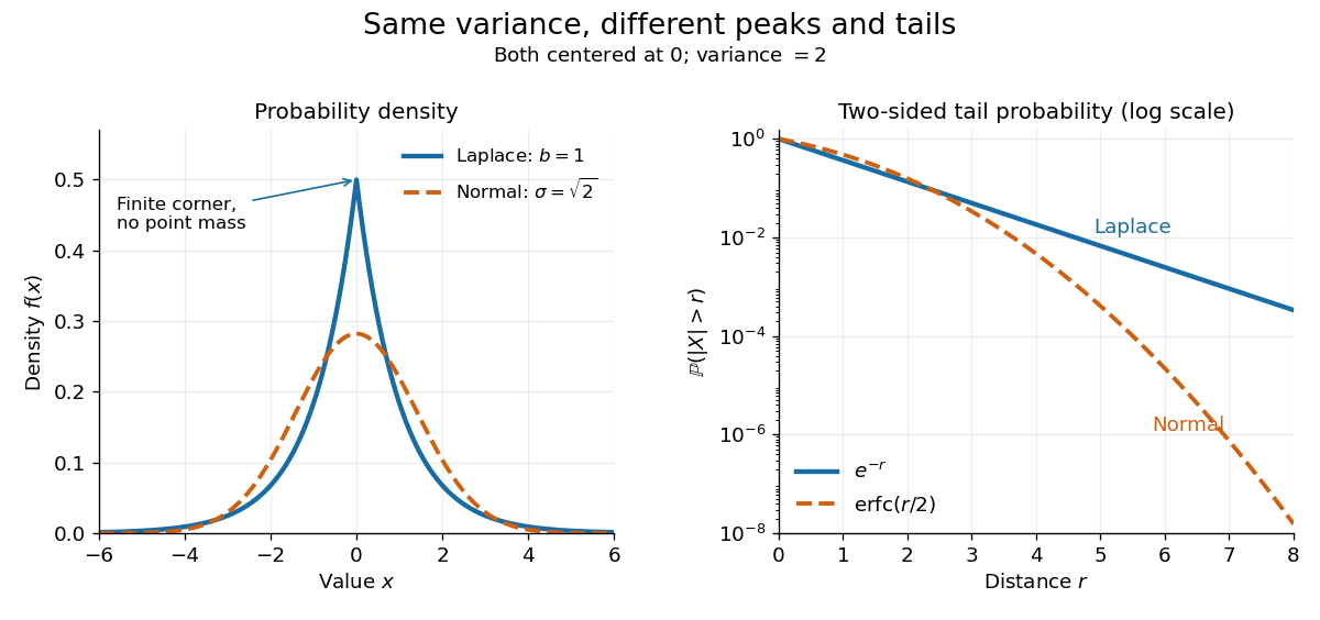
The figure compares a Laplace distribution with $\mu =0$, $b=1$ against a normal distribution with mean zero and standard deviation $\sigma =\sqrt{2}$: both have variance 2. The right panel uses a logarithmic scale for the two-sided tail probability $\mathbb{P}(|X|>r)$. Its straight Laplace distribution curve comes from $e^{-r}$; the normal distribution tail falls faster. Thus values far from the center can be more plausible under a Laplace distribution even after matching the variance. These are theoretical curves, not measured frequencies. The tails still have exponential decay; this is not a heavy-tailed distribution in the convention requiring every positive exponential moment to diverge.

Integrating either half of the probability density function gives the cumulative distribution functionIn particular $F(\mu )=1/2$. The basic moments areThus the scale is the expected value of the absolute distance from the center, and is not the standard deviation. ^[ref] A short way to obtain the moments is to note that $R=|X-\mu |$ has an exponential distribution with rate $1/b$: $\mathbb{P}(R>r)=e^{-r/b}$ for $r\ge 0$. Integrating gives $\mathbb{E}R=b$ and $\mathbb{E}{R}^2=2b^2$; the symmetric distribution gives the centered first moment zero.

The exponential distribution with rate $c>0$ has densityIt is the gamma distribution with shape one.

The Gamma distribution with shape $a>0$ and rate $r>0$ has probability density functionThe gamma function normalizes its integral to one. Its mean is $a/r$ and its variance is $a/r^2$, obtained by integrating powers of $x$. At $a=1$ it is the exponential distribution; integer $a$ gives the waiting time to the $a$th event of a rate-$r$ Poisson process. Independent gamma variables with the same rate add their shapes. Some sources use scale $1/r$ instead of rate, so the parameter convention must accompany the formula.

A probability density function represents probabilities as areas under a nonnegative measurable function. For a real random variable with an absolutely continuous probability distribution, it satisfiesfor every Borel set $A$. Its height is probability per unit of the outcome variable, not the probability of that exact outcome. Thus a probability density function may exceed one, while the probability of a singleton is zero. NIST describes the interval-probability interpretation through integration. ^[ref].

For the example $f_Y(y)=2y$ on $[0,1]$, $f_Y(0.8)=1.6$, but $\mathbb{P}(Y=0.8)=0$ and $\mathbb{P}(0.7<Y<0.9)=0.9^2-0.7^2=0.32$. The cumulative distribution function is $F_Y(y)=y^2$ within that interval, connecting density height to the local accumulation rate.

Changing the scale changes the density height. If $Z=100Y$, then $f_Z(z)=f_Y(z/100)/100=z/5000$ on $[0,100]$. At the corresponding value $z=80$, its height is $0.016$, while $\mathbb{P}(70<Z<90)=0.32$ is unchanged. The factor $1/100$ compensates for the wider integration variable. This is a change of variables, not a change in the underlying probabilities.

A probability density function is determined only almost everywhere: changing its values on a Lebesgue measure zero set changes no probabilities. The Cantor distribution has no such representation, and a mixed probability distribution can have both a point mass and a density component, so differentiating its cumulative distribution function does not recover all its mass.

An isomorphism of Banach spaces is a bijective bounded linear map whose inverse is bounded. The bounded inverse theorem makes boundedness of the inverse automatic.

Two distinct reduced fractions with denominators below $N$ differ by more than $1/N^2$, so an interval of radius $1/(2N^2)$ contains at most one.

A continued-fraction matrix packages the recurrences for continued fraction convergents into matrix multiplication. PutIf $p_n/q_n=[a_0;\dots ,a_n]$, with $p_{-2}=0$, $p_{-1}=1$, $q_{-2}=1$ and $q_{-1}=0$, thenFor $n=0$ the identity is immediate. Right multiplication by $M(a_n)$ replaces the first column by $a_n$ times the old first column plus the old second column, proving the convergent recurrences by mathematical induction.

Each factor has determinant $-1$, so $p_n{q}_{n-1}-p_{n-1}{q}_n=(-1{)}^{n+1}$. Any common divisor of $p_n$ and $q_n$ must therefore divide $1$. Thus each continued fraction convergent is a fraction with coprime numerator and denominator.

A simple continued fraction terminates exactly when its value is rational. For a reduced rational $p/q$, each reciprocal step is one step of the Euclidean algorithm and replaces the denominator by a strictly smaller nonnegative remainder.

A context-free grammar is in Chomsky normal form when every production has the form $A\to BC$ or $A\to a$, with $A,B,C$ nonterminals and $a$ a terminal. If the empty word belongs to the language, one commonly also permits the exceptional rule $S\to ϵ$ under the usual restriction on the start symbol.

Two grammars are equivalent when they generate the same formal language.

A parse tree places the start symbol at its root, the symbols on the right side of a production at the children of its left-side nonterminal, and terminal symbols at its leaves. Reading the leaves from left to right gives the tree's yield.

A grammar derivation is a finite sequence of words in which each step replaces one occurrence of a production's left side by its right side. A leftmost derivation always replaces the leftmost available nonterminal.

A level $L_{\lambda }$ is a coding level when $\lambda$ is a limit ordinal, the representation of every well-order code in $L_{\lambda }$ is below $\lambda$, and every ordinal below $\lambda$ has a well-order code in $L_{\lambda }$.

A well-order code represents a pair $(D,R)$ with $D\subseteq \omega$ and $R\subseteq D\times D$ such that $R$ is a strict well-order of $D$. Its rank is the unique countable ordinal isomorphic to $(D,R)$. Allowing a subset $D$ is essential: $D=\varnothing$ codes zero, a finite $D$ codes a finite ordinal, and infinite subsets code infinite countable ordinals.

Both the domain and relation can be recorded by bits in a real number, using a fixed enumeration of pairs of natural numbers. Different well-order codes can represent the same ordinal; changing the labels of the elements changes the code while preserving its order type.

A condensation sentence is a fixed first-order sentence $\sigma$ such that every transitive set satisfying $\sigma$ is $L_{\lambda }$ for a limit ordinal $\lambda$. It combines a sufficiently strong finite fragment of set theory, the assertion that every set is constructible, and the absence of a largest ordinal.

For an expanding spatially flat universe with constant $w>-1$ and $a(t_0)=1$,It vanishes at the finite past time $t_{\ast }=t_0-2/[3(1+w)H_0]$.

A hydrodynamic mode is a long-wavelength collective mode whose decay rate tends to zero because of a conservation law. Coupling to fast nonconserved variables renormalizes its diffusivity and eigenvector.