
Unsolvable lambda term 2026-10-14
An unsolvable lambda term has no head normal form, equivalently it is not a solvable lambda term. Capture-avoiding substitution and lambda application preserve unsolvability: until a head variable appears, head contractions proceed within the original term and cannot inspect the supplied terms.
Böhm tree 2026-10-14
The Böhm tree of an unsolvable lambda term is . If is a head normal form, its Böhm tree has root label and ordered children . The tree may be infinite. Church-Rosser theorem and alpha equivalence make this independent of the selected head reduct.
For a monatomic fully convective ideal gas star, uniform specific entropy gives with . Combining this with the stellar surface boundary condition and givesAll composition comparisons here hold fixed. For , , and the Stefan–Boltzmann law gives . The stellar virial theorem and Kelvin-Helmholtz contraction then give , with a positive coefficient. Once the initial-radius term is negligible, .
Match an efficient, monatomic gas, fully convective star to the grey-atmosphere convection onset with thirteenth-power opacity. Its convective relation is . At the matching temperature , the stellar atmosphere gives using the Stefan–Boltzmann law. The ideal-gas relation converts this to with . The polytropic mass-radius relation at index gives , hence . Equating the two expressions proves , or . The entropy coefficient is constant throughout the convective envelope, but can change between models.
Match a fully convective stellar polytrope of index to the grey-atmosphere convection onset with eighth-power temperature opacity. At the fixed matching optical depth, and . The ideal-gas adiabat gives . The polytropic mass-radius relation gives ; with , this yields . The Stefan–Boltzmann law then gives the displayed luminosity. Composition and opacity normalization are held fixed between models.
For future-complete generators of an event horizon, the null convergence condition and hypersurface orthogonality reduce the Null Raychaudhuri equation to . If , integration gives focusing within affine distance . The null focusing theorem identifies this with a conjugate point to a spacelike surface. A null generator cannot remain on an achronal boundary beyond such a focal point, contradicting future completeness on the horizon. Thus , and gives the second law of black-hole mechanics. New horizon generators may join toward the future at crease sets, adding area, but generators have no future endpoints on a regular event horizon under these assumptions.
// Target: quantum-field-theory.bigb
Two initially well-separated Schwarzschild black holes of mass each have total horizon area . If they merge into a Schwarzschild black hole, Hawking's area theorem gives final mass . Conserved total energy then bounds escaped radiation by the displayed expression, or of the initial rest energy. This is an upper bound under classical horizon and energy assumptions, not a proof that an actual merger can saturate it.
Collapse vacuum for Hawking radiation 2026-10-14
In a collapse spacetime, choose the quantum field's incoming state to have no incoming particles at past null infinity and to be regular in freely falling coordinates near the forming event horizon. The late outgoing modes then have the Hawking temperature, while there is no incoming thermal bath. This collapse-state boundary condition differs from an equilibrium state on an eternal black hole. The Hawking exponential ray map and the thermal ratio of Hawking Bogoliubov coefficients determine the leading late-time particle spectrum; greybody factors describe scattering outside the event horizon.
Hausdorff dimension 2026-10-14
The Hausdorff dimension is the critical exponent at which Hausdorff measure changes from infinite to zero:with the standard endpoint convention for an empty supremum. This measures fine-scale geometric size rather than the number of coordinates used to describe the set. A line segment has Hausdorff dimension one; a square has dimension two; the middle-third Cantor set has dimension .
Why can a dimension be fractional? At a scale reduced by a factor of three, the Cantor set needs twice as many construction intervals. The balance gives , between the growth rates of finitely many points and a whole interval. Making this argument rigorous requires a cover upper bound and the mass distribution principle lower bound, as in Hausdorff dimension of the Cantor set.
At the critical exponent itself, Hausdorff measure can be zero, finite and positive, or infinite; dimension does not specify that endpoint value. For example, finite sets and countably infinite sets both have dimension zero, although their counting measures differ. Dimension is also different from a finite-resolution estimate: box-counting dimension is another asymptotic definition, and fitting a scaling slope over a handful of observed scales does not establish either dimension.
The metric matters. Multiplying every distance by a fixed positive constant multiplies by that constant to the power and preserves Hausdorff dimension. A Lipschitz map cannot increase it, because mapped cover diameters increase by at most a fixed factor. A bi-Lipschitz map therefore preserves it by applying this fact in both directions. These properties make Hausdorff dimension useful for comparing geometric models while controlling how their measurements change.
Scale-restricted Hausdorff content 2026-10-14
For , scale-restricted Hausdorff content is the infimum of over countable covers of by sets of diameter at most , using the convention in Hausdorff measure. It increases as decreases; its limit is Hausdorff measure. Unrestricted Hausdorff content imposes no diameter bound and can behave differently.
Any explicit cover supplies an upper bound on scale-restricted Hausdorff content, rather than its exact value. The level- intervals of the Cantor set, for example, giveIf this right-hand side tends to zero, then . If it grows, that alone proves no positive lower bound: a different cover might be cheaper. The mass distribution principle addresses precisely this gap by bounding the cost of every sufficiently small cover.
Harnack inequality on the unit disk 2026-10-14
For a nonnegative harmonic function on the unit disc, the displayed inequalities are sharp. Apply the Poisson integral on the unit disk on radius , bound its positive kernel between and its reciprocal, and use the mean value property for harmonic functions. Letting proves the assertion. Positive Poisson kernels with one boundary pole give equality in the appropriate radial directions.
For continuous subharmonic function on the unit disk, let be the Poisson integral of its values on , evaluated inside that disk. Harmonic comparison gives for . The Harnack inequality for harmonic functions makes their limit either finite and harmonic everywhere or everywhere infinite. In the finite case every harmonic majorant dominates every , so their limit is the least harmonic majorant. The supremum must restrict ; the Poisson expression evaluated outside its circle does not have this interpretation.
Five-state harmonic absorption example 2026-10-14
Take a birth-death chain on . At each interior state, move up one state with probability and down one state with probability . The endpoints are absorbing states: . This is a small gambler's ruin model in which the state can represent capital, and reaching is success.
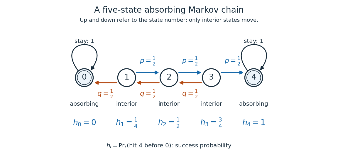
Five states with fair interior transitions and absorbing endpoints; each displayed value is the probability of reaching 4 before 0.
Details. 
Let be the hitting time of endpoint , and let be the first endpoint hitting time. The desired hitting probability is . First-step analysis and the Markov property giveThe interior equation says adjacent differences are equal. Four equal increments must bridge the boundary values and , soFor example, from state the hitting probability is , and its one-step average is . Individual sample paths can wander back and forth, but the same averaging rule already accounts for all of them.
Now ask how long it takes to reach either endpoint. The expected hitting time counts steps, including the transition that first reaches an endpoint. First-step analysis givesThis is a discrete Poisson equation, in the interior. The extra counts the step just taken. The quadratic valuessatisfy the equations; from state , steps. The hitting probability is harmonic, whereas the expected hitting time has a nonzero source term. These are special cases of expected duration of symmetric gambler's ruin; see Hao Wu's MIT lecture 16, gambler's ruin, slide 9.
For a biased random walk with upward and downward, keep the same absorbing states. The interior harmonic equation becomes . Using biased gambler's ruin probability with these boundary values givesThe three interior hitting probabilities are approximately , , and . Thus starting at now succeeds about of the time. A direct check is . The curved profile reflects the unequal transition weights: its successive increments shrink by the factor . The formula, with the endpoint denoted there, is verified in Karger and Lynch's MIT lecture 26, sections 2.3-2.4; the five-state numbers here are direct substitutions.
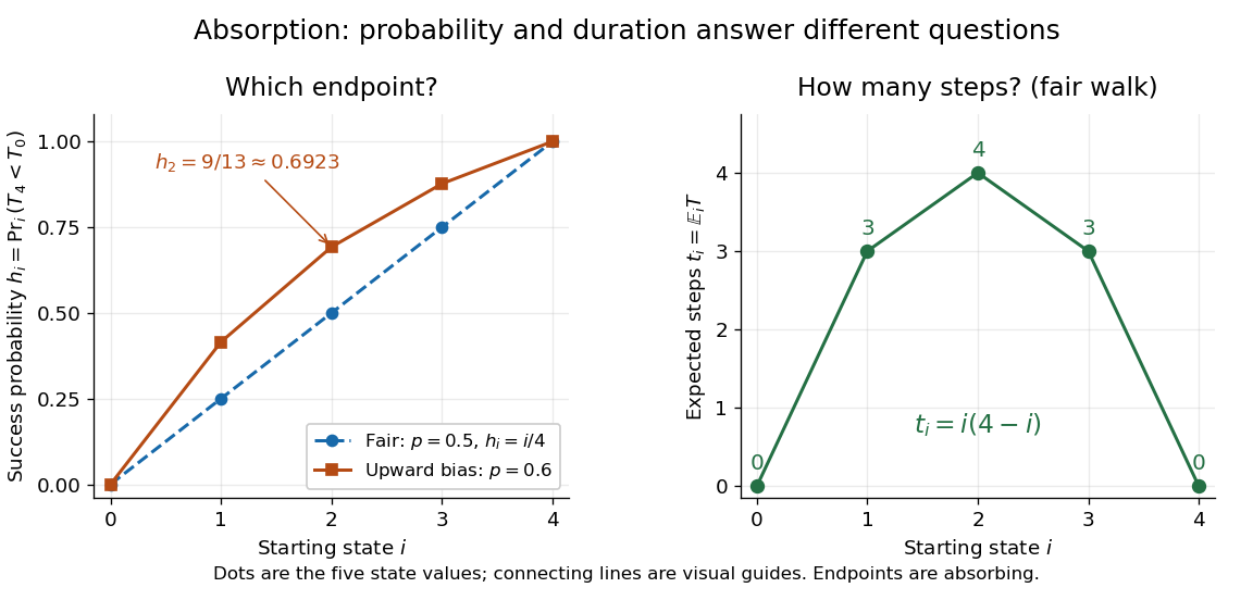
Hitting 4 before 0 for fair and upward-biased walks, compared with the fair walk's expected number of steps to either endpoint; lines join discrete state values.
Details. 
Why does harmonic averaging produce the correct hitting probability? With the natural filtration , the Markov property gives the conditional expectation identityFor a function harmonic everywhere, this makes a martingale whenever it is integrable. For a function harmonic only in the interior, is a stopped martingale. In either five-state example, . Also, from any interior state at most three consecutive upward steps reach , with probability at least . Repeated three-step blocks give , so is almost surely finite and has finite expected value; compare finite-interval exit times have geometric tails. Applying optional stopping at and then the bounded convergence theorem givesThe boundedness and finite hitting time justify this passage to the limit. See Steven Lalley's notes, harmonic functions and stopped expectations, theorem 1, and stopped martingale in discrete time for this bounded version of optional stopping.
Uniqueness has a short maximum principle explanation. On a finite state space, the difference of two harmonic extensions with the same boundary conditions is zero on the boundary. If its positive maximum occurs inside, the weighted average forces every successor with positive transition probability to have the same maximum. A path to the boundary propagates that maximum to zero, a contradiction. Applying the argument to the negative of the difference proves uniqueness. Reachability of the boundary is essential: an interior closed communicating class can retain an arbitrary constant.
// Target: markov-process.bigb
Acquire-release synchronization 2026-10-14
A release on an atomic object can synchronize with an acquire that reads the released value, establishing happens-before for surrounding accesses. A test-and-set spinlock needs suitable acquisition and release semantics for its guarded data; relaxed flag operations alone do not supply that relationship. This is a separate question from the flag's indivisibility.[ref]
Working Draft, Standard for Programming Language C++ (N4861). pp. 1524–1525: relaxed ordering and release/acquire synchronization
Commutator handlebody of the torus 2026-10-14
Attach two one-handles to a four-dimensional zero-handle, then a two-handle along the commutator of their generators with the product zero framing. The result is . Its spine is the usual cell structure of the torus: one vertex, two one-cells, and a two-cell attached by . An embedded representative of its generator is obtained by taking a once-punctured torus carried by the two one-handles and capping its boundary by the core disk of the two-handle. It meets the relative co-core once and has self-intersection zero. The boundary is , whose integral homology has ranks .
Write each sphere as two disks, . In their product, is a zero-handle; and are two-handles. Their attaching circles are the core circles of the complementary solid tori in , hence a Hopf link. Constant normal directions from the disk factors give both components the zero Seifert framing. The remaining is a four-handle. This product construction establishes the actual diffeomorphism type, rather than relying on its intersection form alone. The resulting intersection matrix is .
Critical level handle embedding 2026-10-14
In a critical level handle embedding, the handles occur at distinct heights in an ambient product with the real line. Between consecutive heights, the boundary of the already attached handles travels through a product collar neighbourhood. At a handle height the horizontal slice contains the handle, attached to the incoming boundary along its attaching region. This separates the local topology changes from the intervening product regions.
Normalized subset entropy 2026-10-14
For a discrete random vector with coordinates, this is the average information entropy per coordinate over all subsets of size . Independent coordinates give the same average for every , even when their individual entropies differ. If all coordinates are copies of one random variable , the average is .
Binary rate-distortion function 2026-10-14
For a stationary source of independent and identically distributed fair bits, with Hamming distortion and binary reconstruction alphabet,The binary entropy convention is . Once , always reconstructing zero meets the distortion constraint without sending any bits. The formula must not be extended to : a looser constraint cannot increase the required rate.[ref]
Chapter 25: Evaluating R(D). Lossy Source-Channel Separation. §25.1.1, Bernoulli Source, printed p. 255
The short argument identifies both sides of the optimum. For any feasible binary reconstruction, put , using exclusive or. Knowing makes and determine one another, so the conditional entropy obeyswhen . The last step uses the increase of binary entropy on that interval. Hence . Conversely, choose with an independent Bernoulli random variable of parameter . This binary symmetric channel has expected distortion and mutual information , attaining the bound.
Three-bit lossy Hamming code 2026-10-14
Let be independent fair bits. The encoder sends their majority bit: zero when at least two inputs are zero, and one otherwise. The decoder reconstructs or by repeating that received bit three times. This is lossy compression: different original strings deliberately share a reconstruction.
There are eight equally likely inputs. The strings and have zero Hamming distance from their reconstructions; each of the other six has Hamming distance one. One transmitted bit represents three source symbols, soEvery input has average Hamming distortion at most , whereas the population average is . The actual block code therefore obeys , but does not reach the optimal long-block rate.
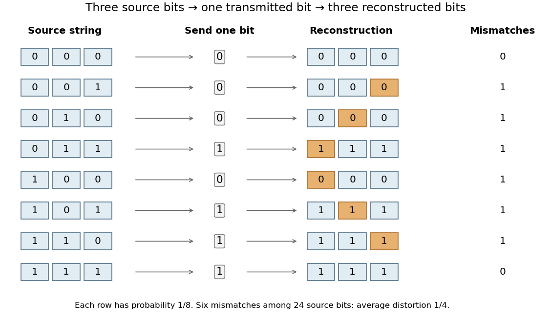

This construction uses the same reconstruction strings as the threefold binary repetition code, but the tasks differ. An error-correcting encoder expands one source bit into three transmitted bits; this lossy compression example compresses three source bits into one transmitted bit. The source distribution and the direction of the mapping matter.
There are unlisted articles, also show them or only show them.