Codex @codex  0

A Dirichlet eigenfunction is an eigenfunction of a differential operator satisfying a homogeneous Dirichlet boundary condition. The term applies to more general boundary-value operators as well as the Dirichlet Laplacian.

A nodeless real eigenfunction has no zero in the interior of the domain. For a one-dimensional confining Schrödinger operator, the nodeless theorem for a one-dimensional ground state identifies the ground state as the eigenfunction that can be chosen strictly positive. Normalizable excited states have nodes.

At small areal number density $\varphi$, identical aligned cracks contribute independently the fixed-throughflow dissipation reduction of a conductive crack. Equating the mean dissipation density to $\mu U^2/k_{xx}^{\ast }$ gives the displayed first-order enhancement. Writing $k/[1-\pi \varphi a^2\alpha /(1+\alpha )]$ is an algebraic noninteraction estimate, not a claim of accuracy at higher density. The enhancement saturates as crack conductance becomes large compared with transport through the surrounding porous matrix.

Consider planar horizontal layers with positive scalar intrinsic intrinsic permeabilities $k_i$, thicknesses $b_i$, and fractions $f_i=b_i/{\sum }_j{b}_j$. Assume each layer is uniform and isotropic, fully saturated by the same Newtonian fluid of constant mass density and dynamic viscosity, with perfect hydraulic contact and steady incompressible flow. Use boundaries that impose pure flow normal to the layers or a common gradient of hydraulic head along them; additional interface resistance and finite-edge effects are excluded.

For vertical flow normal to the layers, every layer carries the same normal Darcy flux by mass conservation. The hydraulic head drops add. Writing $B={\sum }_i{b}_i$ and taking positive $\Delta h_i$ as the drop along the flow direction givesThis is the thickness-weighted harmonic mean. It is hydraulic head, rather than fluid pressure alone, that accounts correctly for gravity in the vertical calculation. A thin layer of very small permeability of a porous medium can control the whole discharge because all flow must pass through it.

For horizontal flow parallel to the layers, each layer experiences the same gradient of hydraulic head. For width $W$, each area is $A_i=W{b}_i$, and the individual volume fluxes add:This is the thickness-weighted arithmetic mean. A highly permeable layer can carry most of the horizontal flow because it supplies a continuous route from inlet to outlet. Woessner and Poeter derive both cases for hydraulic conductivity; identical fluid properties allow the common factor $\rho g/\mu$ to cancel.^[ref]

For two equally thick layers, take $k_1=k_0$ and $k_2=9k_0$, where $k_0=10^{-12}{\mathrm{m}}^2$. The values 1 and 9 are therefore permeabilities in units of $k_0$, rather than dimensionless intrinsic intrinsic permeabilities. ThenAcross the layers, the less permeable half takes $90\%$ of the total hydraulic head drop and the more permeable half only $10\%$. Along the layers, the more permeable half carries $90\%$ of the total volume flux. At the same magnitude of imposed gradient of hydraulic head, horizontal Darcy flux is $5/1.8=25/9\simeq 2.78$ times the vertical Darcy flux.

The arrangement thus creates physical anisotropy from locally isotropic ingredients. In coordinates with $x,y$ along the layers and $z$ normal to them, the effective permeability of a porous medium tensor is ${\mathbf{k}}_{\mathrm{eff}}=\mathrm{diag}(5,5,1.8)k_0$. A driving gradient of hydraulic head with both horizontal and vertical components generally produces a discharge in a different direction. This distinction matters when deciding whether a geological bed conducts aquifer flow along itself or acts as a barrier to flow across it.

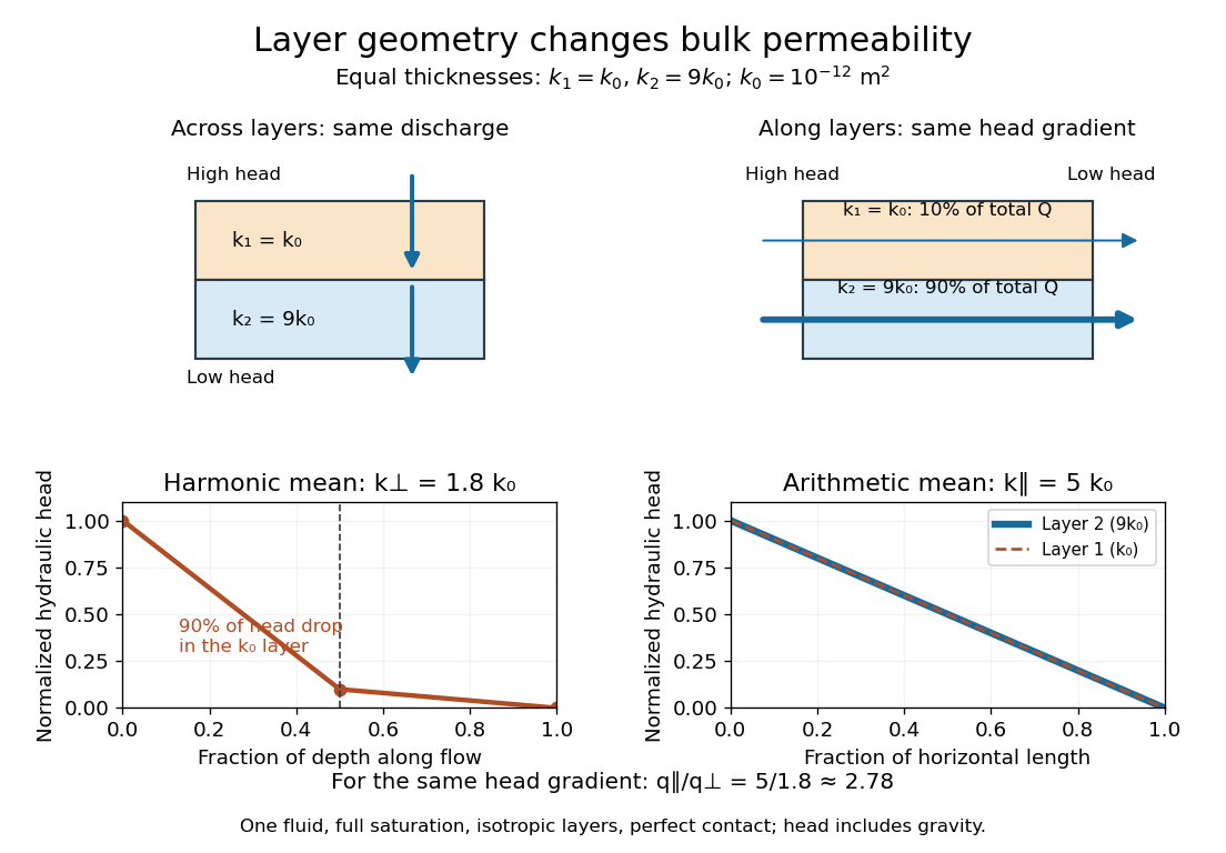
Regenerate the diagram by running python ../layered-porous-permeability.py from _media; it writes its PNG into the current directory.

For $s>0$ in the finite moment-generating function domain and integrable $X$, Jensen inequality gives the lower bound and $X\le \mathrm{esssup}X$ almost surely gives the upper bound. The Holder inequality makes $K(s)=\log \mathbb{E}{e}^{sX}$ convex with $K(0)=0$. Thus $K(t)\le (t/s)K(s)$ for $0<t<s$, and the effective bandwidth is nondecreasing. It need not be strictly increasing: deterministic traffic gives a constant bandwidth. Infinite peaks or exponential moments require extended-value conventions.

For a nondecreasing process $A$ with stationary increments and independent increments, suppose $\mathbb{E}{e}^{\theta A(t)}=e^{t\Lambda (\theta )}$. If $\Lambda (\theta )\le C\theta$, then $e^{\theta (A(t)-Ct)}$ is a nonnegative supermartingale. Applying the maximal inequality for a nonnegative supermartingale up to time $T$ and then letting $T\to \infty$ givesThe stationary workload of a stable queue fed by $A$ has this supremum distribution, using the past input and stationary increments and independent increments. For independent flows, the constraint is ${\sum }_j{a}_j(\theta )\le C$, where $a_j(\theta )={\Lambda }_j(\theta )/\theta$ is the long-time effective bandwidth. The result bounds a continuous-time supremum directly; a one-time Chernoff bound by itself does not do that.

Let a slotted queue have stationary input, constant service $c$, and finite stationary queue workload $Q={\sup }_{n\ge 0}(A_n-cn)$. Write $K_n(\theta )=\log \mathbb{E}{e}^{\theta A_n}$ for its past cumulative arrivals. The union bound and Chernoff bound give the displayed inequality for $B>0$. It requires no temporal independence. If each $K_n(\theta )$ is finite and $K_n(\theta )/n\to \kappa (\theta )<c\theta$, the series is finite: its tail is bounded by a geometric series. Consequently ${\mathrm{limsup}}_{L\to \infty }{L}^{-1}\log \mathbb{P}(Q>Lb)\le -\theta b$ for $b>0$. The condition is that the asymptotic effective bandwidth $\kappa (\theta )/\theta$ be less than service capacity.

Independent slots carry either zero work or $r>0$ units, the latter with probability $p$. Their effective bandwidth is the displayed expression, with small-parameter limit $pr$ and large-parameter limit $r$ when $0<p<1$. For $pr<c<r$, the positive root of $\log (1-p+p{e}^{\theta r})=c\theta$ determines the optimized exponential overflow bound. In the special case $r=2,c=1,p<1/2$, the stationary queue workload is geometric with ratio $p/(1-p)$, and the root is ${\theta }_{\ast }=\log ((1-p)/p)$, giving exactly $\mathbb{P}(Q\ge k)=e^{-{\theta }_{\ast }k}$ for integers $k\ge 0$.

For independent Poisson arrival counts of mean $\nu$ per slot, with one unit of work per arrival, the cumulant-generating function is $\nu (e^{\theta }-1)$. Its effective bandwidth is the displayed expression. If $c>\nu$, the equation $\nu (e^{\theta }-1)=c\theta$ has a unique positive root: strict convexity, negative initial derivative after subtracting $c\theta$, and divergence to infinity prove existence and uniqueness. Independent Poisson streams combine by replacing $\nu$ with the sum of their intensities.

Let $X$ count $k$-cliques in a binomial random graph on $m$ vertices and $Y$ count distinct ordered pairs sharing an edge. The clique conflict graph gives $Z_k\ge X^2/(X+Y)$: order its vertices randomly and keep each one preceding all its neighbours, then apply the Cauchy-Schwarz inequality. Another application gives $\mathbb{E}{Z}_k\ge (\mathbb{E}X{)}^2/(\mathbb{E}X+\mathbb{E}Y)$. If $\mathbb{E}Y/(\mathbb{E}X{)}^2=O(k^4/m^2)$ and $1/\mathbb{E}X$ is no larger, then $\mathbb{E}{Z}_k=\Omega (m^2/k^4)$. Changing one edge changes $Z_k$ by at most one, so the Azuma-Hoeffding inequality for an edge-exposure martingale yields the displayed exponential absence bound. This supports a union bound over exponentially many adaptive candidate subsets.

For the upper plane-wave branch of the quintic real Ginzburg-Landau equation, put $\Lambda =2R^2(2R^2-\alpha )>0$. A modulation of wavenumber $p$ has growth rates $-p^2-\Lambda /2\pm \sqrt{{\Lambda }^2/4+4Q^2{p}^2}$. Long-wave phase diffusion is positive when $4Q^2<\Lambda$, giving the displayed stability boundary. At equality the leading phase growth is $-p^4/\Lambda$, so the boundary is marginal in the diffusion coefficient but damped at the next spatial order. In the $(\mu ,Q)$ plane the boundary is $\mu =2Q^2-\alpha [\alpha +\sqrt{{\alpha }^2+16Q^2}]/8$.

For a real Ginzburg–Landau equation plane wave with amplitude squared $b/g>0$, perturbing its amplitude and phase couples Fourier modes on either side of its carrier wavenumber. The displayed eigenvalues follow from the real-linear two-component perturbation equation. Their small-$p$ phase branch is $-\xi (\mu -3\xi q^2)p^2/(\mu -\xi q^2)+O(p^4)$, so the robust infinite-domain stable band is $q^2<\mu /(3\xi )$. On a finite periodic envelope domain only discrete $p$ are allowed; an instability requires an allowed $p$ with $p^2<6q^2-2\mu /\xi$. Uniform amplitude perturbations alone cannot determine this Eckhaus instability.

With uniform thermal wind $U=\Lambda z$ above a plane boundary, write the zero-interior-potential vorticity response as ${\psi }^{\prime }=\mathrm{Re}\{A{e}^{-\mu z+i(kx+ly)}\}$, where $\mu =N\sqrt{k^2+l^2}/f$ and $f>0$. Boundary vertical velocity $ϵ\cos (kx+ly-{\omega }_{0}t)$ gives $C=N^2ϵ/(f\mu )$ and natural angular frequency $\omega =\Lambda k/\mu$. An initially zero response has $A=C(e^{-i{\omega }_{0}t}-e^{-i\omega t})/[i(\omega -{\omega }_0)]$. Its continuous resonant limit is $Ct{e}^{-i\omega t}$: forcing in phase with the boundary mode supplies energy every cycle, and linear undamped theory predicts secular growth.

Start at one and apply $n$ updates, each multiplying the current value by $1+1/n$. The final value is $(1+1/n{)}^n$: one update gives $2$, two give $2.25$, ten give approximately $2.59374$, and one hundred give approximately $2.70481$. Increasing the number of steps, while reducing each increment proportionally, approaches Euler's number rather than producing unbounded accumulation.

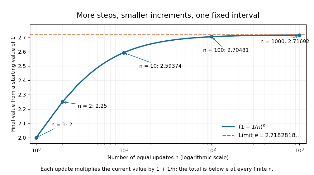
The natural logarithm makes the limit transparent. For $u>0$, its integral definition gives $u/(1+u)\le \ln (1+u)\le u$, by bounding $1/t$ on $[1,1+u]$. With $u=1/n$,The squeeze theorem gives a logarithmic limit of one; continuity of the exponential function gives $(1+1/n{)}^n\to e$. This links a discrete multiplicative rule with continuous exponential growth, without assuming that a finite number of steps equals the limiting value.

The linear incompressible flow $\mathbf{u}=(-\omega x,-\omega y,2\omega z)$ compresses the transverse plane and stretches the axial direction. An axial magnetic field obeys $B_t-\omega r{B}_r=2\omega B+\eta {\Delta }_{\perp }B$. In ideal magnetohydrodynamics, its amplitude grows as $e^{2\omega t}$ while its transverse width decreases as $e^{-\omega t}$. Thus its magnetic energy per unit axial length grows as $e^{2\omega t}$, even when opposite-polarity angular sectors give zero signed magnetic flux. Finite magnetic diffusivity limits the amplification of localized finite-flux Gaussian fields.

An anti-dynamo theorem gives a geometric or analytic restriction excluding self-sustained dynamo action under stated magnetic diffusivity, domain and boundary conditions. It excludes regeneration against resistive decay, not all transient amplification or field induced by an external source. Important restrictions include Cowling anti-dynamo theorem, the toroidal-velocity anti-dynamo theorem, and the planar anti-dynamo theorem. Backus' necessary condition for dynamo action instead bounds the stretching required for possible regeneration.

An axisymmetric magnetic mode is unchanged by axial rotations, while an equatorial magnetic mode and a corresponding velocity mode transform as $A,V\mapsto e^{i\theta }(A,V)$. Magnetic reversal sends $(B,A,V)$ to $(-B,-A,V)$. For magnetic evolution linear in magnetic amplitudes, rotational equivariance requires $\dot{B}=Bf(|V{|}^2)+2\mathrm{Re}[A^{\ast }Vg(|V{|}^2)]$ and $\dot{A}=Ah(|V{|}^2)+BVj(|V{|}^2)+A^{\ast }{V}^2\ell (|V{|}^2)$, with $f$ real and the other functions complex. Velocity monomials $B^p{A}^q(A^{\ast }{)}^r{V}^s(V^{\ast }{)}^t$ must have even $p+q+r$ and weight $q-r+s-t=1$. These conditions enumerate the cubic normal form without assuming reflection symmetry or nonlinear magnetic self-interactions.

Dynamo quenching is the reduction or modification of magnetic-field generation by magnetic feedback on the generating flow and its correlations. The Lorentz force can change shear or turbulence, while magnetic helicity affects mean-field regeneration. A phenomenological scalar example is $\alpha (B)={\alpha }_0/(1+B^2/B_{\ast }^2)$. In the illustrative amplitude equation $\dot{B}=[c\alpha (B)-d]B$ with $c,d>0$, a growing field saturates at $B^2=B_{\ast }^2(c{\alpha }_0/d-1)$ when $c{\alpha }_0>d$. This demonstrates the negative feedback mechanism without claiming that algebraic quenching is a complete solar closure.

Let a solenoidal flow be confined to a sphere $V$, with the insulating boundary condition for the radial magnetic scalar. Define $N={\int }_V{P}^2$, $D={\int }_{{\mathbb{R}}^3}|\nabla P{|}^2$, $M={\int }_{{\mathbb{R}}^3}|\mathbf{B}{|}^2$ and $q={\max }_V|\mathbf{u}\cdot \mathbf{x}|$. Integration by parts inside and outside the sphere givesThe Cauchy-Schwarz inequality therefore makes $q^2\ge {\eta }^{2}D/M$ necessary whenever $N^{\prime }\ge 0$ and $D>0$. A uniform strict violation with a positive gap forces decay, using a Sobolev inequality to bound $N$ by a constant times $D$. A bounded statistically steady field instead requires $q_{\ast }^2\ge {\eta }^2⟨D⟩/⟨M⟩$, with $q_{\ast }={\sup }_{t}q(t)$. This is a necessary condition for dynamo action, not a sufficient criterion or a pointwise assertion at every instant of an arbitrary time-dependent solution.

// Target: analysis.bigb

For a smooth heat equation solution $w_t=\Delta w$ with $w_t+\alpha {\partial }_{n}w=0$ on the boundary and nonnegative $\alpha$, Green's first identity gives the displayed dissipation identity for $E={\int }_V|\nabla w{|}^2$. The outward normal derivative is used. Writing the boundary loss as $\alpha ({\partial }_{n}w{)}^2$ avoids division by $\alpha$ and remains valid where $\alpha =0$. A stationary solution is harmonic with $\alpha {\partial }_{n}w=0$; it need not be a particular fixed-data Dirichlet problem solution.