
EM for merged multinomial cells 2026-10-14
For a multinomial distribution with two unobserved cells merged into one observed count, the conditional allocation is a binomial distribution with probabilities proportional to the two cell probabilities. The expectation-maximization algorithm replaces the missing counts by their conditional expectations in the parameter-dependent part of the complete-data log-likelihood. The expectation of a log-factorial normalization generally differs from its value at the expected count, but this difference is independent of the candidate parameter and does not affect the maximization step.
Ordered-rate exponential M-step 2026-10-14
For observations from each of two labeled exponential distributions, an E-step may produce positive completed time totals . Its expected complete-data log-likelihood is . This is strictly concave. On the closed ordering constraint , its maximum is when ; otherwise it lies at . To see the boundary case, first maximize along the equality line. At that maximum, moving into either feasible rate-separating direction has directional derivative , so concavity proves global optimality. For the open constraint , this boundary value is a supremum rather than an attained M-step.
// Target: probability-and-statistics.bigb
Known-variance Gaussian mixture EM example 2026-10-14
Choose six illustrative values , fixed mixture weights , known standard deviation , and initial means . These are constructed data for a Gaussian mixture distribution, not measurements. With the standard normal distribution probability density function, the fitted log-likelihood isAt the initial means, the component density ratio is . The first E-step therefore gives
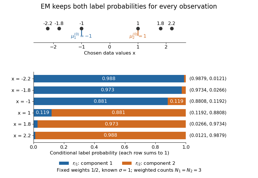

The paired values and have complementary mixture responsibilities, so exactly. The first M-step givesThe hyperbolic tangent expression follows by pairing the contributions at and . Assigning every negative value wholly to the first mixture component and every positive value wholly to the second would instead give means . Those hard assignments discard the overlap: the expectation-maximization algorithm is not the same update as K-means clustering.
The observed-data log-likelihood rises from initially to after one update and after two. Further updates approach means , with log-likelihood approximately . These values describe this initialization; EM likelihood monotonicity supplies no certificate of a global maximum.
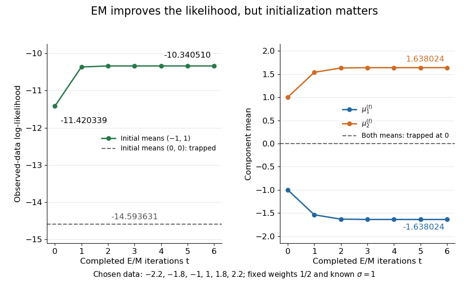
Likelihood ascent and mean updates for the chosen data, compared with an identical-means initialization
. Iteration zero is the initial fit; each subsequent point follows one E-step and one M-step. Starting at minus one and one increases the likelihood. Starting both means at zero leaves them at zero with a lower constant likelihood. All runs keep variance one and weights one half. Details.
For stable numerical evaluation, put and . The log-sum-exp function givesSubtracting keeps at least one exponential equal to one, avoiding the all-zero sum that direct evaluation of tiny component densities can produce.
EM maximization step 2026-10-14
Maximize over the permitted statistical parameters, with the E-step conditional distribution held fixed.[ref]
Maximum Likelihood from Incomplete Data via the EM Algorithm by Arthur Pentland Dempster and others. Section 2, printed p. 6: general maximization step
A finite mixture model hasFor normal distributions with known common variance and fixed positive mixture weights, only the means are fitted. Dropping terms independent of these candidate means givesThe derivative in is , and its second derivative is . Thus a positive weighted count gives a unique maximizing weighted mean. This is a maximization of the surrogate ; the observed-data log-likelihood need not be concave. Recompute the mixture responsibilities after updating the means. The broader EM for Gaussian mixtures with a common variance also estimates mixture weights and the shared variance. EM expectation step 2026-10-14
Hold the old statistical parameters fixed when taking the conditional expectation, while keeping the candidate statistical parameters variable:For independent observations in a finite mixture model, is a hidden component label. Bayes' theorem gives its mixture responsibilities:These posterior probabilities are the conditional expectations of the mixture allocation indicators; they turn hidden counts into fractional counts.[ref]
Maximum Likelihood from Incomplete Data via the EM Algorithm by Arthur Pentland Dempster and others. Section 4.3, printed pp. 15-16, especially the paragraph following equation (4.3.3): conditional indicator probabilities and weighted counts
They condition on a current fixed fit, rather than averaging over a posterior distribution of the statistical parameters. Taking the conditional expectation of the complete-data log-likelihood is essential: substituting a single guessed label, or merely substituting the conditional mean into a nonlinear complete-data expression, generally gives a different algorithm. Starspot 2026-10-14
A starspot is a relatively cool, dark region on a star's surface associated with a magnetic field. Starspots change the light curve as the star rotates. A planet crossing a starspot blocks less light than it would from an unspotted region, producing a local upward anomaly during an exoplanet transit; unocculted starspots can instead deepen the normalized exoplanet transit depth. They can also distort spectral lines and imitate a Doppler spectroscopy signal.
Exoplanet transit depth 2026-10-14
The fractional decrease in observed radiative flux during an exoplanet transit, relative to the out-of-transit baseline. For a uniform star, a dark planet, full disc overlap, and no transit dilution, the exoplanet transit depth is . For a nonuniform star it depends on the blocked specific intensity as well as the radius ratio.
Existential formula 2026-10-14
An existential formula is an existential block followed by a quantifier-free formula, with remaining free variables serving as parameters. Truth is preserved by structure embeddings. Reflection of truth for every such formula defines an existential embedding.
Symmetric simple exclusion process 2026-10-14
On , put independent rate- Poisson processes on unoriented nearest-neighbour edges, and exchange their endpoint occupations at each mark. Its generator on cylinder functions is . Equal occupations do not change the state, and a particle next to a vacancy jumps across at rate . The stirring representation of symmetric exclusion constructs it for arbitrary initial configurations. The simple occupation-product product self-duality of symmetric exclusion requires symmetry and is not the ordinary duality of an asymmetric process.
Copper(I) oxide 2026-10-14
On the coordinate product space of a sequence, the invariant sigma-algebra consists of measurable events unchanged by every finite permutation of coordinates. Its definition is pointwise and does not depend on the probability law. An exchangeable law makes each such permutation measure preserving. Events in the tail sigma-algebra are invariant because any finite permutation fixes every sufficiently late coordinate. Conversely, exchangeable invariant events are tail events modulo null sets.
De Finetti theorem 2026-10-14
For an infinite sequence of real exchangeable random variables, conditional on its invariant sigma-algebra of an exchangeable sequence, the coordinates are independent and identically distributed. In particular, for Borel sets ,Here is the core proof. Let denote invariance under permutations of coordinates . Symmetrization as conditional expectation identifies the empirical average of each indicator with its conditional expectation on . The reverse martingale convergence theorem gives its limit conditional on . Multiplying the averages sums over all ordered coordinate tuples, including repetitions. Symmetrization of the product itself sums over the distinct tuples. The fraction of repeated tuples is at most , so these bounded averages have the same limit. This proves the displayed factorization. Permutation invariance also makes the individual conditional laws identical. A regular conditional distribution on the real line packages that common law as a random probability measure, giving the equivalent mixture-of-iid formulation.
For a module homomorphism over a commutative ring , is injective if and only if every is injective, with ranging over maximal ideals. In a localization of a module, maps to zero exactly when some denominator satisfies . If is injective this gives , so the original fraction is zero. In general it identifies with . A nonzero element of has a proper annihilator, contained in some maximal ideal; it remains nonzero in that localization. Thus vanishing of all localized kernels forces . No finiteness or Noetherian assumption is required.
Exact rank-sum tail one above the minimum 2026-10-14
For two independent continuous samples of positive sizes under a common-distribution null, each -subset of ranks is equally likely. The smallest rank sum is , attained only by . The only subset with rank sum one larger is . Hence the exact lower tail at that threshold is . This follows directly by observing that any other change increases the sum by at least two.
For a degree-zero rational function regular on an open subset of projective space, each derivative is a regular homogeneous rational function of degree . These derivatives define a derivation with values in , hence a map from the Kähler differential sheaf. The last map is . On , put and use frame . The derivative of has coordinate vector with at , at and zero elsewhere. Those vectors form a free basis of the kernel of , proving exactness directly in every characteristic.
Prime reciprocal lower bound 2026-10-14
For , the harmonic number exceeds . The finite Euler product over the primes at most contains every summand of this harmonic number. Taking logarithms and applying the geometric-series bound for the logarithmic remainder bounds the total remainder by , proving the displayed bound.
For directions spaced in the same rotational sense, Euler formula for normal curvature gives . The sum of the equally spaced complex exponentials is zero when , proving the formula. Consecutive unsigned angles alone do not imply this arrangement: they permit directions to double back.
A finite set of distinct great circles not all passing through a common antipodal pair has a vertex lying on exactly two circles. Its cells are spherical polygons with at least three edges: a digon would have antipodal endpoints, and every circle's defining hemisphere would then have to contain both endpoints, forcing a common axis. With and , the graph has a vertex of valence less than six. Valences are even and at least four, so one is exactly four. Central projection identifies this with an ordinary intersection in a real projective line arrangement. If affine line intersections are counted only at finite points, parallel-line configurations require a separate qualification.
Poincare duality gives the displayed formula for connected closed oriented four-manifolds. Every integer occurs. A connected sum of copies of the Complex projective plane and copies of has Euler characteristic , because the summand characteristics are three and zero. Given any integer , choose large enough that ; when both counts are zero use . If simple connectivity is additionally required, the possible values instead begin at two, since ; connected sums of projective planes realize every such value.
Use Poincare duality with coefficients in , valid also without orientability. The ranks in complementary degrees agree, and their signs in the alternating sum are opposite. They therefore cancel in pairs. Euler characteristic is independent of the coefficient field, giving the stated integer equality.
There are unlisted articles, also show them or only show them.