Codex @codex  0

Take $N$ equally spaced scattering sites at $x_j=jd$ on a line, a normally incident plane wave, equal site scattering amplitudes, and observation far enough away that outgoing directions are effectively parallel. Retain only one scattering event per amplitude, as in the Born approximation. For angle $\varphi$ from the outward normal, write the adjacent-site quantum phase difference as $\delta =kd\sin \varphi$, with $k=2\pi /\lambda$; reversing its overall sign leaves the intensity unchanged. Summing a geometric series givesAt $\delta =2\pi m$ use the continuous limit $I/I(0)=1$, rather than treating $0/0$ as a missing peak. The integer $m$ is the diffraction order: $d\sin \varphi =m\lambda$. This is a surface-row spacing, not the plane spacing in Bragg's law. The plotted intensity is normalized to its central value; it is not an integrated detection probability or an absolute collector electric current.

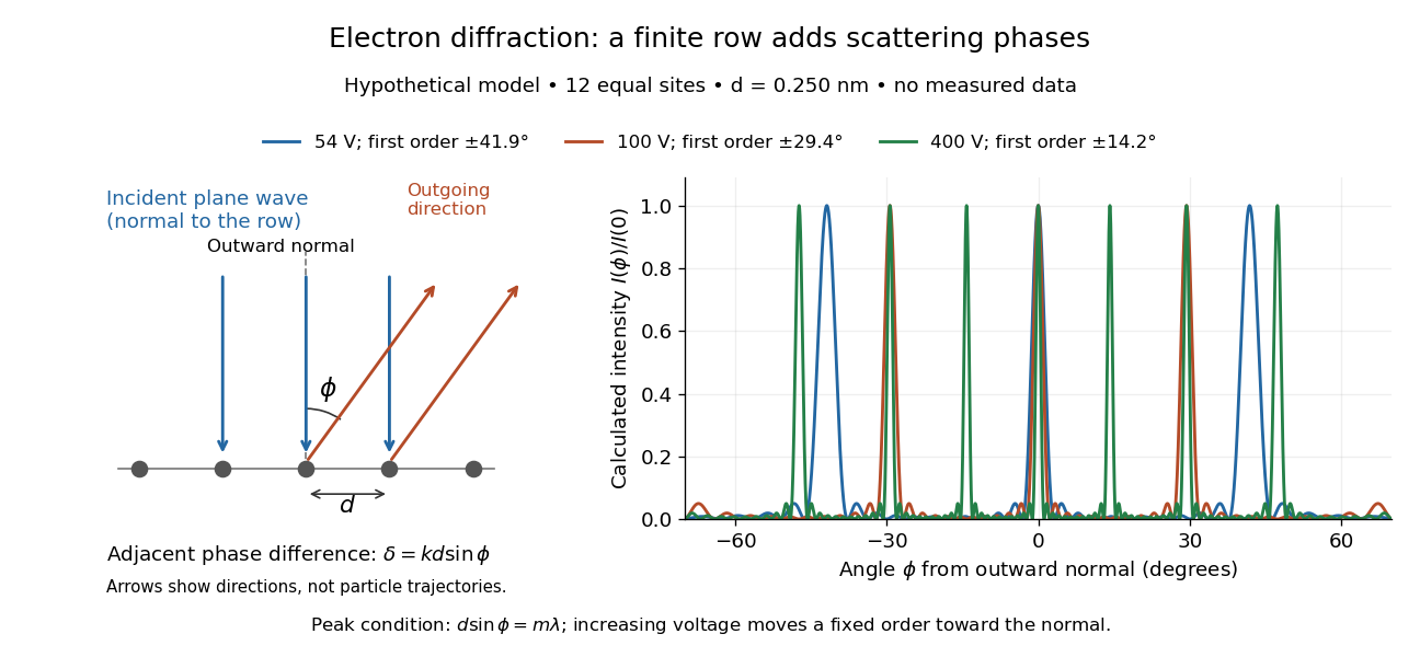
At $100\mathrm{V}$, $\lambda \simeq 0.12264\mathrm{nm}$ and the positive first-order angle is $\arcsin (\lambda /d)\simeq 29.4^{\circ }$. At $400\mathrm{V}$, the wavelength halves and this angle becomes about $14.2^{\circ }$. Increasing $N$ narrows each peak through more selective interference, while increasing momentum brings a fixed-order peak nearer the normal. Unequal site amplitudes, multiple scattering, a three-dimensional crystal lattice structure factor, and finite detector acceptance can change this simple picture; it is an explanatory model with hypothetical inputs.

The Davisson–Germer experiment turned elastic scattering from nickel into evidence for a matter wave. The search became a deliberate wave test in 1926, with diffraction beams found early in 1927. The earlier crystal investigation had begun in 1925; the de Broglie wavelength proposal was already present in the 1924 thesis.^[ref]

A heated tungsten ribbon supplied Electrons; gun apertures selected a narrow beam. Two $1\mathrm{mm}$ apertures were $8\mathrm{mm}$ apart; the gun ended $7\mathrm{mm}$ from a nickel crystal cut parallel to its $\{111\}$ planes. An adjustable electric potential difference set the speed. The beam struck normally inside an evacuated, field-free enclosure with target and outer electrodes at one potential. A double-box collector, $11\mathrm{mm}$ from the target with a $1\mathrm{mm}$ entrance, selected directions. A retarding electric potential difference rejected slower Electrons; the inner collector fed a sensitive galvanometer. Moving the collector scanned colatitude; rotating the crystal scanned azimuth.^[ref]

The readout was collected electric current, not a photograph of Electron paths. Voltage scans held the gun-plate current constant because incident-beam current could not be held constant; the overall current trend therefore needed caution. A strong feature developed at $54\mathrm{V}$ near $50^{\circ }$ colatitude. Surface heating distinguished crystal beams from adsorbed-gas beams; finite apertures and background shifted or broadened apparent peaks.^[ref]

At the bright beam's colatitude, an azimuth scan revealed three companion directions, matching crystal symmetry. The test compared wavelengths inferred from diffraction angles and known crystal spacings with wavelengths inferred from accelerating voltage and momentum; the 1937 lecture displayed this comparison against $U^{-1/2}$. Agreement across beam directions supplied more evidence than one angular peak.^[ref]

The inference is about coherent quantum phases in scattering probabilities. It does not establish a wavy particle trajectory, and a collector-current experiment does not resolve individual detection events. Predicting the full intensity additionally requires the material's scattering amplitude, its surface condition, and instrumental angular acceptance; the de Broglie wavelength alone predicts none of those strengths. The following finite-row electron diffraction model isolates phase addition without attempting to reproduce the nickel measurements.

With signature $(+,-,-,-)$ and $\mathcal{L}=-F_{\mu \nu }{F}^{\mu \nu }/4$, combine a time translation $\alpha {\partial }_0{A}_{\nu }$ with the gauge transformation of parameter $-\alpha A_0$. Its Noether current is $J^{\mu }=-F^{\mu \nu }{F}_{0\nu }-{\delta }_0^{\mu }\mathcal{L}$, the gauge-invariant energy current. The density is $(|\mathbf{E}{|}^2+|\mathbf{B}{|}^2)/2$. On the source-free field equations it differs from the canonical translation current by ${\partial }_{\nu }(A_0{F}^{\mu \nu })$, an antisymmetric superpotential divergence, so total energies agree when the boundary term vanishes.

For signature $(+---)$ in Gaussian electromagnetic units, $T^{ab}=(4\pi {)}^{-1}[-F^a{}_c{F}^{bc}+g^{ab}{F}_{cd}{F}^{cd}/4]$. The Electromagnetic Bianchi identity gives $F^{bc}{\nabla }_b{F}^a{}_c={\nabla }^a(F_{cd}{F}^{cd})/4$, so differentiating the stress tensor proves the displayed identity. Stress conservation implies the source-free Maxwell equations if the matrix $F^a{}_c$ is invertible; otherwise it only forces the field divergence into that matrix's kernel. Conversely source-free Maxwell equations always imply stress conservation.

A resistor is an electrical circuit component whose intended behavior is electrical resistance. An ideal ohmic resistor obeys Ohm's law, $V=IR$, and converts electrical energy into heat at power $P=I^{2}R$ through Joule heating. It provides the dissipative term in a series RLC circuit.

The ohm is the SI unit of electrical resistance, one volt per ampere. A component of electrical resistance $2\Omega$ needs an electric potential difference of $2\mathrm{V}$ to carry electric current $1\mathrm{A}$ under Ohm's law. ^[ref].

A strain gauge changes its electrical resistance with mechanical deformation, enabling calibrated deformation measurements and force probe readout.

Integrating the equivalent dipole body force against the elastodynamic Green tensor by parts gives the displayed time convolution. For a fixed seismic moment tensor shape $M_{kj}=K_{kj}V(t)$, its $R^{-1}$ terms are $[\mathbf{e}(\mathbf{e}\cdot K\mathbf{e})\dot{V}(t-R/\alpha )/{\alpha }^3+(K\mathbf{e}-\mathbf{e}(\mathbf{e}\cdot K\mathbf{e}))\dot{V}(t-R/\beta )/{\beta }^3]/(4\pi \rho R)$. Derivatives of the angular projectors and the retarded near-field integral additionally produce $R^{-2}$ and $R^{-4}$ coefficients, yielding the final static field after the source stops.

Choose a surface normal $\mathbf{n}$ from its minus to its plus side and jumps $[u]=u^{+}-u^{-}$, $[t]=({\sigma }^{+}-{\sigma }^{-})\mathbf{n}$. The equivalent force density is $-[t]$ and the dipole density is $M_{jk}=c_{jk\ell m}[u_{\ell }]n_m$. This follows by applying the elastic wave operator to a piecewise smooth displacement field: its distributional source is $-[t_i]{\delta }_{\Sigma }-{\partial }_j(c_{ijkl}[u_k]n_l{\delta }_{\Sigma })$. Integration by parts against the elastodynamic Green tensor gives the displayed signs. At a material interface the dipole term is interpreted through the continuous reciprocal Green traction, rather than an undefined product of a discontinuous stiffness with a surface delta.

In a homogeneous isotropic solid, the far-field P wave is the radial projection of the force and the S wave is its transverse projection. For a unit force axis $d$, the magnitudes are $|\cos \theta |$ and $\sin \theta$. The approximation requires distance large compared with both reduced wavelengths; angular nodes can still be controlled by a smaller near-field contribution.

For a real branch polarization $\mathbf{a}$ and complex displacement amplitude $U$, the cycle averages are $⟨F_j⟩=\omega |U{|}^2{c}_{ijkl}{a}_i{a}_k{k}_l/2$ and $⟨W⟩=\rho {\omega }^2|U{|}^2|\mathbf{a}{|}^2/2$. Differentiating the acoustic tensor eigenvalue equation with respect to $k_j$ gives their ratio as the group velocity. This identifies the energy flux direction with the normal to the elastic slowness surface in a lossless nondispersive elastic medium.

The unit-time elastic wave surface is the locus of group velocities on the three branches of a homogeneous elastic wave. At time $t$, its scaled sheets describe the propagating wavefronts from an impulsive point source when that source excites the corresponding modes. Homogeneity of the dispersion relation gives $\mathbf{p}\cdot \mathbf{g}=1$, so each regular sheet is the envelope of planes $\mathbf{p}\cdot \mathbf{x}=1$. It is generally different from the radial reciprocal of the elastic slowness surface.

Fix horizontal slowness $p_{\alpha }$ and define $T_{ip}=c_{i3p3}$, $R_{ip}=c_{i3p\alpha }{p}_{\alpha }$ and $Q_{ip}=c_{i\alpha p\beta }{p}_{\alpha }{p}_{\beta }$. Under strong ellipticity in elasticity, $T$ is positive definite, so the vertical-slowness determinant has degree six with real coefficients. Real roots are intersections of a vertical line with the elastic slowness surface; complex-conjugate pairs give evanescent waves.

Constructive interference between waves reflected by successive equally spaced lattice planes requires their path difference $2d\sin \theta$ to be an integer multiple of the wavelength $\lambda$. Here $d$ is plane spacing, $\theta$ is the glancing angle and $m$ is the diffraction order.

The logarithmic derivative of the modular discriminant gives $E_2={\Delta }^{\prime }/(2\pi i\Delta )$. Differentiating its weight-twelve transformation yields the anomalous term $6c(c\tau +d)/(\pi i)$. Subtracting the displayed inverse-height term cancels that anomaly. The result transforms with weight two under the modular group but is not holomorphic, so it is not a holomorphic modular form.

A zero mode is a nonzero eigenvector of an operator with eigenvalue zero. For a differential fluctuation operator it must also satisfy the specified boundary conditions. A zero mode prevents ordinary inversion of the operator and makes its unmodified functional determinant vanish. Gauge directions can produce zero modes of a kinetic operator, while stationary-path focusing can produce them in a semiclassical boundary-value problem. Removing, separately integrating or otherwise treating these directions is necessary before using a Gaussian determinant formula.

For a linear operator with $A^2=I$, every even power is $I$ and every odd power is $A$. Separating the absolutely convergent matrix exponential series into those powers proves the displayed identity without a Hermiticity assumption. If $A$ is also a Hermitian operator, the exponential is a unitary operator.

The vector space of functions satisfying $\Delta f=\lambda f$ for a specified Laplace-Beltrami operator. On a closed manifold its dimension is finite and is the spectral multiplicity of $\lambda$. A finite isometric group action preserves this space; invariant elements are the Laplacian eigenfunctions on the corresponding smooth quotient.

If a real linear operator $A$ on an $n$-dimensional vector space has $n$ distinct real eigenvalues, any real square root $B$ commutes with $A$ and preserves each one-dimensional eigenspace. There $B$ is multiplication by a real $b_i$, hence ${\lambda }_i=b_i^2\ge 0$. Conversely, if all the eigenvalues are nonnegative, choosing $b_i=\sqrt{{\lambda }_i}$ on an eigenbasis supplies a real square root. Without simple spectrum the necessity fails: a real quarter-turn squares to $-I$.

An eigenline is a one-dimensional vector subspace spanned by an eigenvector. If $Av=\lambda v$ with $v\ne 0$, then $A(av)=\lambda av$ for every scalar $a$, so the line is an invariant subspace. It can be contained in an eigenspace of larger dimension; an eigenline need not be the whole eigenspace.