
The given spatial and carrier factors combine into retarded copies of the same random field:On the axis, and . Expand the squared electric-field wave amplitude. Each self term contributes , and the two cross terms together contribute the real part of the full-field correlation. Stationarity and giveIn vacuum, and . Reversing the delay convention replaces by without changing this real-part result. This is the electric-field light intensity convention of the question. For two nonparallel waves it should not automatically be identified with the magnitude of the net Poynting vector; part (d) gives that geometric conversion explicitly.
Take at a fixed reference point, and define the full-field temporal optical coherence function byThe angle brackets denote an ensemble expected value, or a sufficiently long time average when justified. The factor puts in light intensity units for the chosen peak complex-field convention. The normalized first-order optical coherence is for a stationary source.
“Independent of absolute time” means the second moment depends on the time difference but not on the starting time : shifting both observation times by the same amount leaves it unchanged. Together with a constant mean this is second-order or weak stationarity; it does not mean that the random electric field is constant in time. Put . The full-field convention is important: an envelope-only correlation omits and must have that carrier factor restored before deriving optical interference fringes.
The circular eigenmode orthogonal projection matrices obey , and . Define the uniform-medium generatorExpanding its matrix exponential by its power series and using these projection identities givesEquivalently, with , one has , and . This is exactly the corrected matrix of part (d). The entries of have units of inverse length, and the map satisfies , and the homogeneous propagation law .
The extra factor in the printed version violates this last law for nonzero , so it cannot be generated by one constant with the stipulated eigenvalues. The constant- description assumes uniform coefficients and fixed circular eigenmodes.
Write , and . Then and . With and , the corrected matrix becomesThe scalar is a common propagation wave phase and the real rotation matrix rotates the input linear polarization through . There is no attenuation and no generated ellipticity: the field map is a unitary matrix. The two circular eigenmodes accumulate different wave phases, giving circular birefringence and optical activity.
The correct unfactored matrix remains finite where . In contrast, the printed form would give times the rotation matrix, including unphysical divergent gain in this stipulated lossless case. This provides a direct physical check on the correction in part (d).
When are real, and are real. The two opposite circular polarizations retain their wave phases but are attenuated at different wave amplitude rates. This circular dichroism changes the ellipticity without rotating the principal axis of the ellipse.
For input , the corrected Jones matrix givesThe common factor describes the mea wave amplitude attenuation. The factor reflects the sum of the two transmitted modal wave amplitudes; fixes their imbalance and hence the signed ellipticity. The real field has components proportional to and , soThe ellipse's principal axis stays along the original input direction. For large differential optical depth it approaches the less attenuated circular eigenmode. A passive medium has , or , so the growing hyperbolic function factor does not imply net optical gain. Using the printed prefactor would give a spurious extra attenuation inconsistent with the modal laws.
There are errors in the original PDF at this point, not merely in the TeX transcription. The second exponential must denote the eigenvalue , not the propagation coefficient itself. More substantially, the printed prefactor is inconsistent with the stated exponential eigenvalues. It must be . The original's primed Jones-matrix label distinguishes the distributed component from the earlier static matrix; below write to avoid confusing that prime with a derivative.
Complex eigenvalues have no intrinsic largest/smallest ordering, so and are modal labels. Keep the circular eigenvectors fixed, put and , and use the spectral decomposition from part (c):Its diagonal entries are , and its upper off-diagonal entry is . ThereforeWhere , this can be factored asThe unfactored expression is valid even at zeros of the cosine-like factor when is imaginary. The printed expression is times this correct matrix; its eigenvalues are consequently rather than those specified. A second check is , whereas the printed version has determinant . Thus the requested printed identity cannot be proved except in the degenerate case ; the following parts use the consistent propagator.
The normalized circular eigenvectors from part (a) define the orthogonal projection matricesThus the spectral decomposition of the Jones matrix isThis simply substitutes and and makes each eigenmode's wave amplitude transmission explicit.
Take an incident field along , without loss of generality because this component has the same circular eigenmodes for every direction of input linear polarization. Resolve its Jones vector into equal circular components:Using the complex amplitude convention , the real circular contributions areThey counter-rotate and add toIn general the tip traces an ellipse with semiaxis lengths and . Equal transmitted circular wave amplitudes produce a line; removal of one circular mode, or , produces a circle. The special zero-output case has no defined polarization of waves.
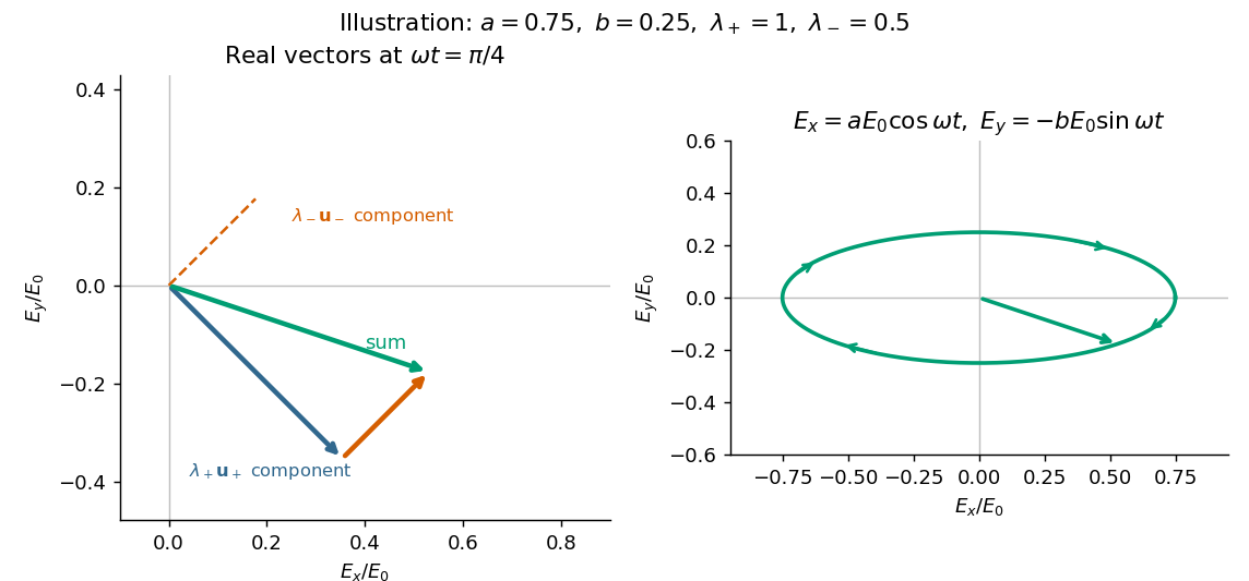

The characteristic polynomial of the given Jones matrix isso a convenient choice of eigenvalue labels isDirect multiplication gives , and . They represent opposite circular polarizations. Since are real, is a Hermitian matrix and both eigenvalues are real, but they need not be positive. A negative eigenvalue adds a wave phase reversal to that mode. The labels are algebraic: is the larger numerical eigenvalue only when . If , the eigenvalue is degenerate and every nonzero Jones vector is an eigenvector; the circular pair remains a valid basis.
Distinguish reflection at the input terminal, reflection at the receiving load, and a returned signal that traverses the free-space link twice. The input antenna is initially matched, so its direct terminal reflection is zero.
In the usual weak-coupling, matched-port two-port network model for the antenna pair, let the forward and reverse wave amplitude transfer coefficients be and . Electromagnetic reciprocity gives equal power transfer factors , where from part (a). The receiving-load reflection returns wave amplitude to the original input port. The load-mismatch contribution to the returned power is thereforeFor fixed gains and impedances this returned power scales as : it contains two link traversals. By contrast, the reflected power at the receiving load before that return traversal is . Calling that local reflected power the power already back in the input line would omit one propagation loss.
The original wording does not specify an antenna scattering model. The boxed result is the load-dependent echo in an ideal matched-port link, with structural scattering and residual input coupling neglected. The actual total input return can include coherent scattering from the receiving antenna even when ; gains and effective areas alone do not specify that background. If “reflected back” means only the direct reflection at the stated matched transmitting antenna, its value is . These meanings should not be conflated; the result requires the two-pass echo interpretation and its stated model.
The transmitting antenna is matched to its input transmission line, so its real terminal electrical resistance is . The identical receiving antenna has the same electrical impedance at the operating frequency. Its available received power for a matched load is the incident energy flux times its antenna effective area:The real receiving load is , so its voltage-wave reflection coefficient relative to is . The fraction of available power delivered to the output line isConsequently, neglecting path losses, mismatch of polarization of an electromagnetic wave and line losses,This is the Friis transmission equation with a receiving impedance-mismatch factor. For fixed , it scales as . That scaling is conditional on holding antenna gain fixed: a fixed physical aperture can instead have , and any wavelength dependence of the impedances also enters the expression. The matched-output check gives .
Now take , with the same angle to the incident direction. The perpendicular direction is and the in-plane transverse direction is . The roles of the two electric dipole populations interchange: electric dipoles radiate at full strength, whereas the observed wave amplitude from a electric dipole is reduced by .
Thus and , givingThis is also obtained by the symmetry , in part (a). For , both planes give the familiar Rayleigh scattering degree of polarization : the diffuse signal is unpolarized forward and fully linearly polarized at right angles. At a dark direction with zero denominator, no degree of polarization can be measured.
Work in the dilute, single-scattering limit and add the diffuse scattered light intensities of randomly positioned particles. The incident unpolarized light has equal, mutually uncorrelated and electric components. Each particle therefore has an induced electric dipole moment along its permitted axis, with the same mean squared magnitude proportional to .
For an observer in direction , choose transverse unit directions in the scattering plane and perpendicular to it. The electric dipole radiation field is proportional to the transverse projection of the electric dipole. Hence an electric dipole contributes a wave amplitude factor along , while a electric dipole contributes its full wave amplitude along .
Let collect the common incident light intensity, electric polarizability, distance and frequency factors. ThenThe two components are uncorrelated, so the coherency matrix is diagonal in this basis. The degree of polarization isA signed degree of linear polarization, defined positive perpendicular to the scattering plane, has the same expression without the absolute value. The dominant direction is when , and when the inequality reverses. If the denominator vanishes there is no scattered signal and its degree of polarization is undefined. A coherent exactly forward component, including the transmitted incident beam, is not part of this diffuse-intensity calculation; random particle positions do not by themselves destroy forward optical coherence.
Write a nonzero vacuum plane electromagnetic wave with wavevector , where is a unit propagation direction. Its propagation Lorentz four-vector is , or, up to a scalar normalization in any one frame, . It is null because .
Choose coordinates and Minkowski metric . With the supplied three-dimensional boost formulas, a consistent convention assigns the printed array to upper-index components,The index conventions for the electromagnetic field tensor then require and when both indices are lowered. The printed lower-index label therefore cannot be kept together with its electric signs and a forward propagation vector in this convention.
This is not merely an arbitrary overall sign. For a valid forward wave with , and , multiplying the printed array, unchanged, by gives an component , rather than zero. One consistent repair is to retain the printed array as and contract with . Equivalently, lower both tensor indices before forming the contraction asked for in the question.
Using that corrected lower-index tensor givesTo establish both electric and magnetic transversality, include the dual electromagnetic field tensor. Choose and ; lowering both indices then givesThe source-free plane-wave Maxwell equations are precisely the pair of covariant conditionsTheir temporal components give and . Their spatial components give the associated amplitude and orientation relations, and .
To see the Lorentz covariance explicitly, let . It is a covector, so if in one inertial frame, its Lorentz transformation is also zero in every other inertial frame. The same is true of . Since the transformed wave still has and , their temporal components implyHere , rather than a vector renormalized to have temporal component one in every frame, is the actual Lorentz four-vector; multiplying a zero contraction by a nonzero normalization does not affect the argument.
Finally, the two scalar perpendicularity statements alone are not equivalent to one tensor contraction. They do not enforce the amplitude relation between and . Conversely alone cannot exclude a longitudinal magnetic field: adding leaves its cross product unchanged. For a genuine source-free plane electromagnetic wave, the remaining Maxwell equations supply that missing constraint, and both tensor contractions vanish. This qualification and the corrected index placement are necessary for the intended invariance argument.
Let be the boost velocity, and decompose the fields into components parallel and perpendicular to it. The parallel components are unchanged. The perpendicular components obeyAll vectors inside these expressions are perpendicular to . Thus , and similarly for . In the difference of squares, the mixed terms cancel becauseIt follows thatAdding the unchanged parallel components provesFor the mixed dot product, expand directly. The terms and vanish. The remaining cross-product identity isHenceParallel-perpendicular mixed dot products are zero in both frames, soRotations also preserve these two expressions, completing the proof for proper Lorentz transformations. The second expression is a pseudoscalar under spatial parity, but is invariant under the boosts at issue here.
These results also follow from tensor contractions. In the convention used below, and . The numerical sign of the latter depends on the chosen orientation of the dual electromagnetic field tensor, while its invariance under proper Lorentz transformations does not.
A distinct classical Thomson scattering window requires two separated scales:To remove that window, the binding frequency must be comparable with or greater than the Compton scattering recoil scale. Thus the formal condition for bound-electron scattering without a Thomson frequency window isUsing the stipulated approximate electron mass , and givesThe dimensions are . The inequality denotes a scale comparison, not a uniquely specified spring constant or a sharp transition.
There is also a physical limitation to the question's premise. Compton scattering does not begin discontinuously at ; recoil corrections grow as photon energy approaches the rest energy. If , the assumed nonrelativistic binding model is itself no longer reliable. The calculation therefore locates where no well-separated classical Thomson scattering range exists; it cannot establish a literal direct transition of a real strongly bound system using this oscillator equation alone.
Put , where is the binding spring constant rather than an optical wavenumber. The steady complex amplitude solution of the forced Lorentz oscillator model isThe acceleration complex amplitude is . HenceThis is the scattering cross-section of a harmonically bound charge. The displacement and induced electric dipole moment are parallel to the incident linear polarization, and integrating their dipole radiation over all directions gives the total cross section above.
For , binding dominates andrecovering Rayleigh scattering with static electric polarizability . For , inertia dominates: , so its second time derivative becomes frequency independent andThis is a classical Thomson scattering regime only while . Exactly at , an undamped driven oscillator has no finite steady-state amplitude; the divergent formula must not be used. Finite damping and radiation reaction regulate the physical resonant response. Coherent contributions from many charges in an extended medium can also require a structure calculation rather than multiplying this single-charge result by a particle count.
Past exam of the optics and electrodynamics course of the University of Cambridge 2019 Section B B5 Thomson limit Created 2026-10-18 Updated 2026-10-20
Thomson scattering describes the low-recoil scattering of electromagnetic radiation by a free charge. For charge and mass , the weak incident field gives peak acceleration . The mean Larmor formula power is thereforeThere is no binding force to introduce a characteristic frequency. Dividing by the same incident light intensity gives the Thomson cross-section:For an electron, the length inside parentheses is the classical electron radius. The cross section has units and is independent of wavelength in this classical limit. The driven velocity must remain small compared with , and must make Compton recoil kinematics negligible.
In Rayleigh scattering, a small bound system develops an induced electric dipole moment . Well below its binding resonances, the electric polarizability is approximately its static value , independent of frequency. The mean radiated power and incident light intensity areDividing gives the total scattering cross sectionThis Rayleigh scattering wavelength dependence comes from the two time derivatives of an oscillating electric dipole moment, whose radiated field is proportional to . It requires the same scatterer with approximately constant low-frequency electric polarizability; resonances and strong optical dispersion invalidate the simple fourth-power law.
Denote the orbit radius by here to distinguish it from observation distance; it is the quantity called in this part of the paper. WriteFor observation at spherical coordinates , measured from the orbit normal,The acceleration magnitude is constant, . Therefore the radiation pattern of a circularly moving nonrelativistic charge isTime averaging removes the azimuthal dependence. The axial intensity is twice the equatorial intensity, and no direction has zero mean intensity: the instantaneous dipole axis continually rotates. This is also the sum of the two orthogonal linear-oscillation patterns with their relative phase quadrature. At equal radius and linear-oscillation amplitude, the total mean power is twice the linear result. The calculation requires ; relativistic synchrotron radiation is outside this approximation.
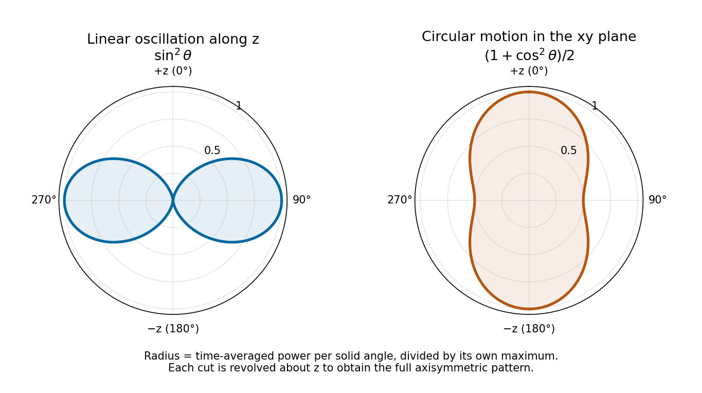
Normalized angular power for linear oscillation and nonrelativistic circular motion, with angle measured from the same z axis
. Details. 
There are unlisted articles, also show them or only show them.